注意
跳到結尾以下載完整的範例程式碼。
從顏色列表建立色圖#
如需建立和操控色圖的更多詳細資訊,請參閱在 Matplotlib 中建立色圖。
可以使用 LinearSegmentedColormap.from_list 方法,從顏色列表建立色圖。您必須傳遞定義從 0 到 1 的顏色混合的 RGB 元組列表。
建立自訂色圖#
也可以為色圖建立自訂對應。這是透過建立字典來完成的,該字典指定 RGB 通道如何從色圖的一端變更到另一端。
範例:假設您希望紅色在底部一半從 0 增加到 1,綠色在中間一半做相同的事情,藍色在頂部一半做相同的事情。然後您會使用
cdict = {
    'red': (
        (0.0,  0.0, 0.0),
        (0.5,  1.0, 1.0),
        (1.0,  1.0, 1.0),
    ),
    'green': (
        (0.0,  0.0, 0.0),
        (0.25, 0.0, 0.0),
        (0.75, 1.0, 1.0),
        (1.0,  1.0, 1.0),
    ),
    'blue': (
        (0.0,  0.0, 0.0),
        (0.5,  0.0, 0.0),
        (1.0,  1.0, 1.0),
    )
}
如果如同此範例,r、g 和 b 元件中沒有不連續性,則它非常簡單:每個元組的第二個和第三個元素是相同的 -- 稱之為 "y"。第一個元素("x")定義了從 0 到 1 的整個範圍的內插區間,並且它必須跨越整個範圍。換句話說,x 的值將 0 到 1 的範圍分割成一組區段,而 y 提供每個區段的端點顏色值。
現在考慮綠色,cdict['green'] 表示:
0 <=
x<= 0.25,y為零;沒有綠色。0.25 <
x<= 0.75,y從 0 到 1 線性變化。0.75 <
x<= 1,y保持在 1,完全綠色。
如果有不連續性,則會稍微複雜一些。將 cdict 中給定顏色的每個列中的 3 個元素標記為 (x, y0, y1)。然後,對於介於 x[i] 和 x[i+1] 之間的值,顏色值會介於 y1[i] 和 y0[i+1] 之間進行內插。
回到食譜範例
cdict = {
    'red': (
        (0.0,  0.0, 0.0),
        (0.5,  1.0, 0.7),
        (1.0,  1.0, 1.0),
    ),
    'green': (
        (0.0,  0.0, 0.0),
        (0.5,  1.0, 0.0),
        (1.0,  1.0, 1.0),
    ),
    'blue': (
        (0.0,  0.0, 0.0),
        (0.5,  0.0, 0.0),
        (1.0,  1.0, 1.0),
    )
}
並查看 cdict['red'][1];因為 y0 != y1,它表示對於從 0 到 0.5 的 x,紅色會從 0 增加到 1,然後它會跳下來,因此對於從 0.5 到 1 的 x,紅色會從 0.7 增加到 1。當 x 從 0 到 0.5 時,綠色會從 0 遞增到 1,然後跳回 0,並且當 x 從 0.5 到 1 時,會遞增回 1。
以上嘗試顯示,對於 x 在範圍 x[i] 到 x[i+1] 中時,內插會在 y1[i] 和 y0[i+1] 之間進行。因此,永遠不會使用 y0[0] 和 y1[-1]。
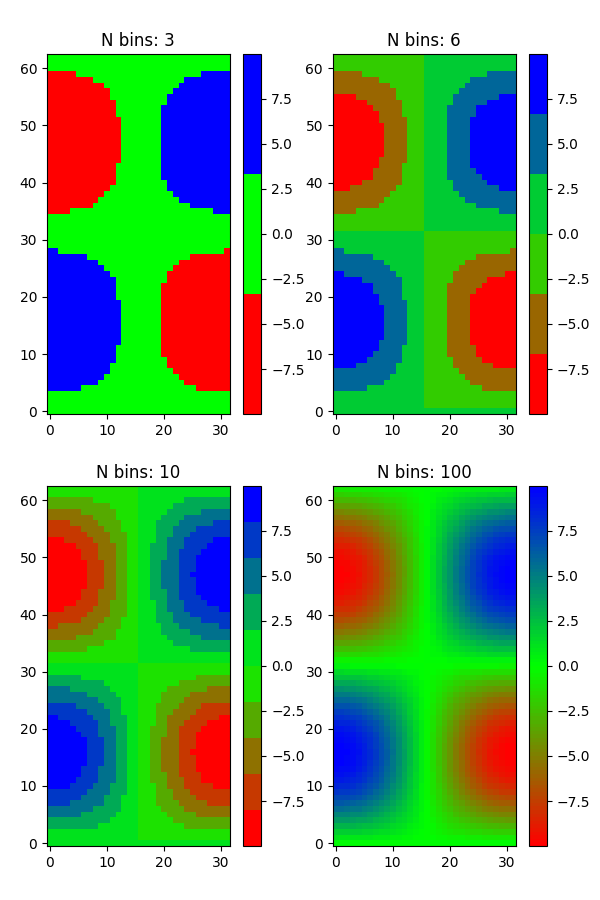
來自列表的色圖#
colors = [(1, 0, 0), (0, 1, 0), (0, 0, 1)]  # R -> G -> B
n_bins = [3, 6, 10, 100]  # Discretizes the interpolation into bins
cmap_name = 'my_list'
fig, axs = plt.subplots(2, 2, figsize=(6, 9))
fig.subplots_adjust(left=0.02, bottom=0.06, right=0.95, top=0.94, wspace=0.05)
for n_bin, ax in zip(n_bins, axs.flat):
    # Create the colormap
    cmap = LinearSegmentedColormap.from_list(cmap_name, colors, N=n_bin)
    # Fewer bins will result in "coarser" colomap interpolation
    im = ax.imshow(Z, origin='lower', cmap=cmap)
    ax.set_title("N bins: %s" % n_bin)
    fig.colorbar(im, ax=ax)
自訂色圖#
cdict1 = {
    'red': (
        (0.0, 0.0, 0.0),
        (0.5, 0.0, 0.1),
        (1.0, 1.0, 1.0),
    ),
    'green': (
        (0.0, 0.0, 0.0),
        (1.0, 0.0, 0.0),
    ),
    'blue': (
        (0.0, 0.0, 1.0),
        (0.5, 0.1, 0.0),
        (1.0, 0.0, 0.0),
    )
}

cdict2 = {
    'red': (
        (0.0, 0.0, 0.0),
        (0.5, 0.0, 1.0),
        (1.0, 0.1, 1.0),
    ),
    'green': (
        (0.0, 0.0, 0.0),
        (1.0, 0.0, 0.0),
    ),
    'blue': (
        (0.0, 0.0, 0.1),
        (0.5, 1.0, 0.0),
        (1.0, 0.0, 0.0),
    )
}

cdict3 = {
    'red': (
        (0.0, 0.0, 0.0),
        (0.25, 0.0, 0.0),
        (0.5, 0.8, 1.0),
        (0.75, 1.0, 1.0),
        (1.0, 0.4, 1.0),
    ),
    'green': (
        (0.0, 0.0, 0.0),
        (0.25, 0.0, 0.0),
        (0.5, 0.9, 0.9),
        (0.75, 0.0, 0.0),
        (1.0, 0.0, 0.0),
    ),
    'blue': (
        (0.0, 0.0, 0.4),
        (0.25, 1.0, 1.0),
        (0.5, 1.0, 0.8),
        (0.75, 0.0, 0.0),
        (1.0, 0.0, 0.0),
    )
}

# Make a modified version of cdict3 with some transparency
# in the middle of the range.
cdict4 = {
    **cdict3,
    'alpha': (
        (0.0, 1.0, 1.0),
        # (0.25, 1.0, 1.0),
        (0.5, 0.3, 0.3),
        # (0.75, 1.0, 1.0),
        (1.0, 1.0, 1.0),
    ),
}
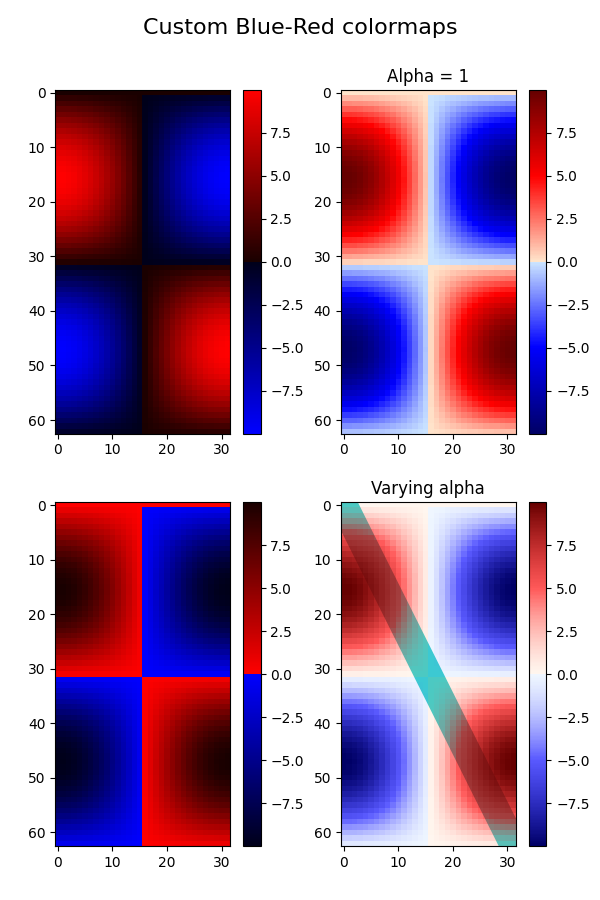
現在我們將使用此範例來說明處理自訂色圖的 2 種方式。首先,最直接和明確的方式
blue_red1 = LinearSegmentedColormap('BlueRed1', cdict1)
其次,明確建立地圖並註冊。與第一種方法類似,此方法適用於任何類型的 Colormap,而不僅僅是 LinearSegmentedColormap
mpl.colormaps.register(LinearSegmentedColormap('BlueRed2', cdict2))
mpl.colormaps.register(LinearSegmentedColormap('BlueRed3', cdict3))
mpl.colormaps.register(LinearSegmentedColormap('BlueRedAlpha', cdict4))
使用 4 個子圖建立圖表
fig, axs = plt.subplots(2, 2, figsize=(6, 9))
fig.subplots_adjust(left=0.02, bottom=0.06, right=0.95, top=0.94, wspace=0.05)

im1 = axs[0, 0].imshow(Z, cmap=blue_red1)
fig.colorbar(im1, ax=axs[0, 0])

im2 = axs[1, 0].imshow(Z, cmap='BlueRed2')
fig.colorbar(im2, ax=axs[1, 0])

# Now we will set the third cmap as the default.  One would
# not normally do this in the middle of a script like this;
# it is done here just to illustrate the method.

plt.rcParams['image.cmap'] = 'BlueRed3'

im3 = axs[0, 1].imshow(Z)
fig.colorbar(im3, ax=axs[0, 1])
axs[0, 1].set_title("Alpha = 1")

# Or as yet another variation, we can replace the rcParams
# specification *before* the imshow with the following *after*
# imshow.
# This sets the new default *and* sets the colormap of the last
# image-like item plotted via pyplot, if any.
#

# Draw a line with low zorder so it will be behind the image.
axs[1, 1].plot([0, 10 * np.pi], [0, 20 * np.pi], color='c', lw=20, zorder=-1)

im4 = axs[1, 1].imshow(Z)
fig.colorbar(im4, ax=axs[1, 1])

# Here it is: changing the colormap for the current image and its
# colorbar after they have been plotted.
im4.set_cmap('BlueRedAlpha')
axs[1, 1].set_title("Varying alpha")

fig.suptitle('Custom Blue-Red colormaps', fontsize=16)
fig.subplots_adjust(top=0.9)

plt.show()
腳本總執行時間: (0 分鐘 2.166 秒)