pcolormesh#

axes.Axes.pcolormesh 可讓您產生 2D 影像樣式的繪圖。請注意，它比類似的 pcolor 快。

import matplotlib.pyplot as plt
import numpy as np

from matplotlib.colors import BoundaryNorm
from matplotlib.ticker import MaxNLocator

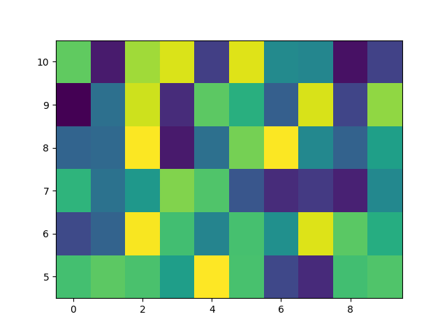
基本 pcolormesh#

我們通常透過定義四邊形的邊緣和四邊形的值來指定 pcolormesh。請注意，在這裡 *x* 和 *y* 在各自的維度中比 Z 多一個元素。

np.random.seed(19680801)
Z = np.random.rand(6, 10)
x = np.arange(-0.5, 10, 1)  # len = 11
y = np.arange(4.5, 11, 1)  # len = 7

fig, ax = plt.subplots()
ax.pcolormesh(x, y, Z)

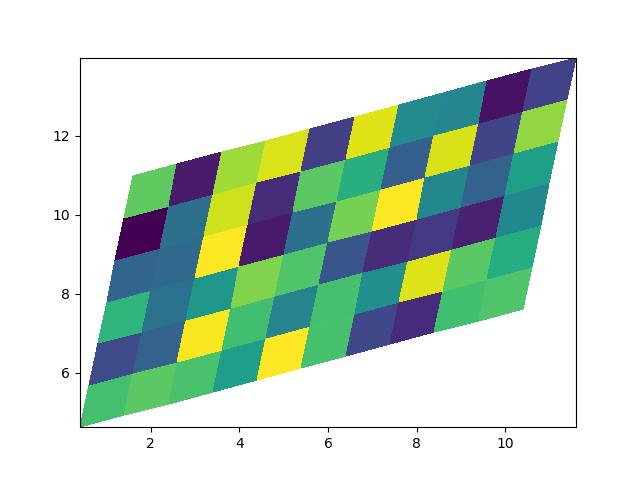
非線性 pcolormesh#

請注意，我們也可以為 *X* 和 *Y* 指定矩陣，並且具有非線性四邊形。

x = np.arange(-0.5, 10, 1)  # len = 11
y = np.arange(4.5, 11, 1)  # len = 7
X, Y = np.meshgrid(x, y)
X = X + 0.2 * Y  # tilt the coordinates.
Y = Y + 0.3 * X

fig, ax = plt.subplots()
ax.pcolormesh(X, Y, Z)

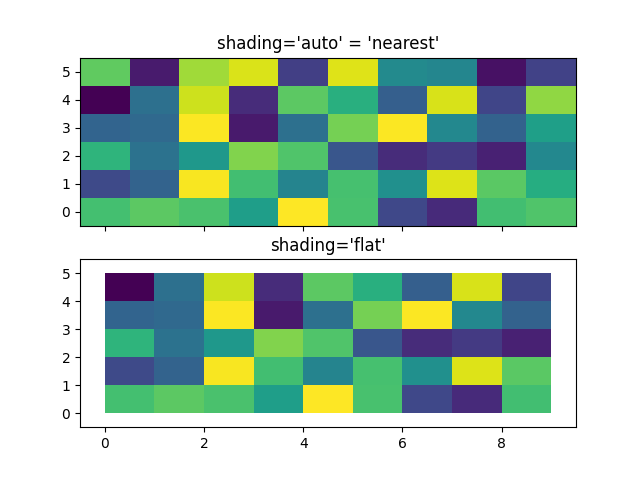
置中座標#

通常，使用者希望將與 *Z* 相同大小的 *X* 和 *Y* 傳遞給 axes.Axes.pcolormesh。如果傳遞了 shading='auto'（由 rcParams["pcolor.shading"] （預設值：'auto'）設定的預設值），這也是允許的。在 Matplotlib 3.3 之前，shading='flat' 會捨棄 *Z* 的最後一欄和一列，但現在會產生錯誤。如果這真的是您想要的，請手動捨棄 Z 的最後一列和一欄

x = np.arange(10)  # len = 10
y = np.arange(6)  # len = 6
X, Y = np.meshgrid(x, y)

fig, axs = plt.subplots(2, 1, sharex=True, sharey=True)
axs[0].pcolormesh(X, Y, Z, vmin=np.min(Z), vmax=np.max(Z), shading='auto')
axs[0].set_title("shading='auto' = 'nearest'")
axs[1].pcolormesh(X, Y, Z[:-1, :-1], vmin=np.min(Z), vmax=np.max(Z),
                  shading='flat')
axs[1].set_title("shading='flat'")

shading='auto' = 'nearest', shading='flat'

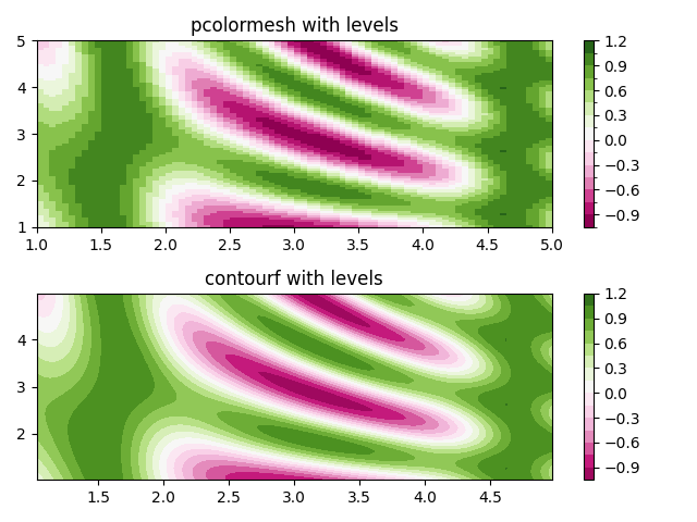
使用 Norm 建立水平#

示範如何組合正規化和色彩映射實例，以在 axes.Axes.pcolor、axes.Axes.pcolormesh 和 axes.Axes.imshow 類型繪圖中繪製「水平」，其方式與 contour/contourf 的水平關鍵字引數類似。

# make these smaller to increase the resolution
dx, dy = 0.05, 0.05

# generate 2 2d grids for the x & y bounds
y, x = np.mgrid[slice(1, 5 + dy, dy),
                slice(1, 5 + dx, dx)]

z = np.sin(x)**10 + np.cos(10 + y*x) * np.cos(x)

# x and y are bounds, so z should be the value *inside* those bounds.
# Therefore, remove the last value from the z array.
z = z[:-1, :-1]
levels = MaxNLocator(nbins=15).tick_values(z.min(), z.max())


# pick the desired colormap, sensible levels, and define a normalization
# instance which takes data values and translates those into levels.
cmap = plt.colormaps['PiYG']
norm = BoundaryNorm(levels, ncolors=cmap.N, clip=True)

fig, (ax0, ax1) = plt.subplots(nrows=2)

im = ax0.pcolormesh(x, y, z, cmap=cmap, norm=norm)
fig.colorbar(im, ax=ax0)
ax0.set_title('pcolormesh with levels')


# contours are *point* based plots, so convert our bound into point
# centers
cf = ax1.contourf(x[:-1, :-1] + dx/2.,
                  y[:-1, :-1] + dy/2., z, levels=levels,
                  cmap=cmap)
fig.colorbar(cf, ax=ax1)
ax1.set_title('contourf with levels')

# adjust spacing between subplots so `ax1` title and `ax0` tick labels
# don't overlap
fig.tight_layout()

plt.show()

pcolormesh with levels, contourf with levels

參考資料

此範例中顯示了以下函式、方法、類別和模組的使用方式

腳本總執行時間：（0 分 3.622 秒）

由 Sphinx-Gallery 產生之畫廊