具有誤差帶的曲線

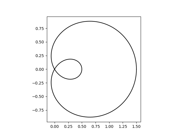
此範例說明如何在參數化曲線周圍繪製誤差帶。

參數化曲線 x(t)、y(t) 可以直接使用 plot 來繪製。

import matplotlib.pyplot as plt
import numpy as np

from matplotlib.patches import PathPatch
from matplotlib.path import Path

N = 400
t = np.linspace(0, 2 * np.pi, N)
r = 0.5 + np.cos(t)
x, y = r * np.cos(t), r * np.sin(t)

fig, ax = plt.subplots()
ax.plot(x, y, "k")
ax.set(aspect=1)

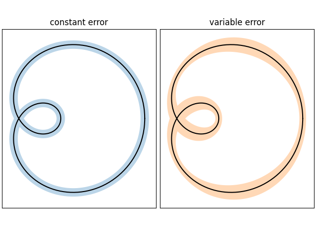
誤差帶可以用來表示曲線的不確定性。在此範例中，我們假設誤差可以用純量 err 來表示，此純量描述每個點垂直於曲線的不確定性。

我們使用 PathPatch 將此誤差視覺化為路徑周圍的彩色帶。路徑是從兩個路徑分段 (xp, yp) 和 (xn, yn) 建立，這兩個分段以與曲線 (x, y) 垂直的 +/- err 位移。

注意：這種使用 PathPatch 的方法適用於 2D 中的任意曲線。如果您只有標準的 y 對 x 繪圖，您可以使用更簡單的 fill_between 方法 (另請參閱 填滿兩條線之間的區域)。

def draw_error_band(ax, x, y, err, **kwargs):
    # Calculate normals via centered finite differences (except the first point
    # which uses a forward difference and the last point which uses a backward
    # difference).
    dx = np.concatenate([[x[1] - x[0]], x[2:] - x[:-2], [x[-1] - x[-2]]])
    dy = np.concatenate([[y[1] - y[0]], y[2:] - y[:-2], [y[-1] - y[-2]]])
    l = np.hypot(dx, dy)
    nx = dy / l
    ny = -dx / l

    # end points of errors
    xp = x + nx * err
    yp = y + ny * err
    xn = x - nx * err
    yn = y - ny * err

    vertices = np.block([[xp, xn[::-1]],
                         [yp, yn[::-1]]]).T
    codes = np.full(len(vertices), Path.LINETO)
    codes[0] = codes[len(xp)] = Path.MOVETO
    path = Path(vertices, codes)
    ax.add_patch(PathPatch(path, **kwargs))


_, axs = plt.subplots(1, 2, layout='constrained', sharex=True, sharey=True)
errs = [
    (axs[0], "constant error", 0.05),
    (axs[1], "variable error", 0.05 * np.sin(2 * t) ** 2 + 0.04),
]
for i, (ax, title, err) in enumerate(errs):
    ax.set(title=title, aspect=1, xticks=[], yticks=[])
    ax.plot(x, y, "k")
    draw_error_band(ax, x, y, err=err,
                    facecolor=f"C{i}", edgecolor="none", alpha=.3)

plt.show()

參考

此範例顯示下列函數、方法、類別和模組的使用

• matplotlib.patches.PathPatch

• matplotlib.path.Path

標籤：元件：錯誤 繪圖類型：線條 層級：中級