陰影範例

範例示範如何製作類似 Mathematica 或 通用繪圖工具的陰影浮雕圖。

import matplotlib.pyplot as plt
import numpy as np

from matplotlib import cbook
from matplotlib.colors import LightSource


def main():
    # Test data
    x, y = np.mgrid[-5:5:0.05, -5:5:0.05]
    z = 5 * (np.sqrt(x**2 + y**2) + np.sin(x**2 + y**2))

    dem = cbook.get_sample_data('jacksboro_fault_dem.npz')
    elev = dem['elevation']

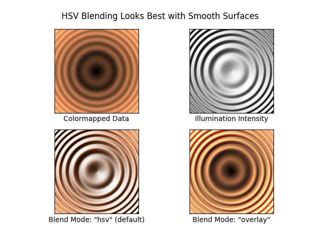
    fig = compare(z, plt.cm.copper)
    fig.suptitle('HSV Blending Looks Best with Smooth Surfaces', y=0.95)

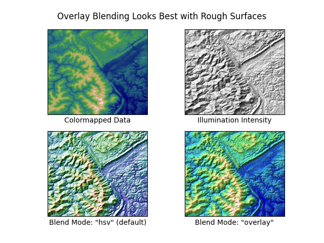
    fig = compare(elev, plt.cm.gist_earth, ve=0.05)
    fig.suptitle('Overlay Blending Looks Best with Rough Surfaces', y=0.95)

    plt.show()


def compare(z, cmap, ve=1):
    # Create subplots and hide ticks
    fig, axs = plt.subplots(ncols=2, nrows=2)
    for ax in axs.flat:
        ax.set(xticks=[], yticks=[])

    # Illuminate the scene from the northwest
    ls = LightSource(azdeg=315, altdeg=45)

    axs[0, 0].imshow(z, cmap=cmap)
    axs[0, 0].set(xlabel='Colormapped Data')

    axs[0, 1].imshow(ls.hillshade(z, vert_exag=ve), cmap='gray')
    axs[0, 1].set(xlabel='Illumination Intensity')

    rgb = ls.shade(z, cmap=cmap, vert_exag=ve, blend_mode='hsv')
    axs[1, 0].imshow(rgb)
    axs[1, 0].set(xlabel='Blend Mode: "hsv" (default)')

    rgb = ls.shade(z, cmap=cmap, vert_exag=ve, blend_mode='overlay')
    axs[1, 1].imshow(rgb)
    axs[1, 1].set(xlabel='Blend Mode: "overlay"')

    return fig


if __name__ == '__main__':
    main()

• 
• 

參考文獻

此範例中顯示了以下函式、方法、類別和模組的使用方式

• matplotlib.colors.LightSource

• matplotlib.axes.Axes.imshow / matplotlib.pyplot.imshow