繪製影像的多種方式

在 Matplotlib 中繪製影像最常見的方式是使用 imshow。以下範例示範 imshow 的許多功能以及您可以建立的許多影像。

import matplotlib.pyplot as plt
import numpy as np

import matplotlib.cbook as cbook
import matplotlib.cm as cm
from matplotlib.patches import PathPatch
from matplotlib.path import Path

# Fixing random state for reproducibility
np.random.seed(19680801)

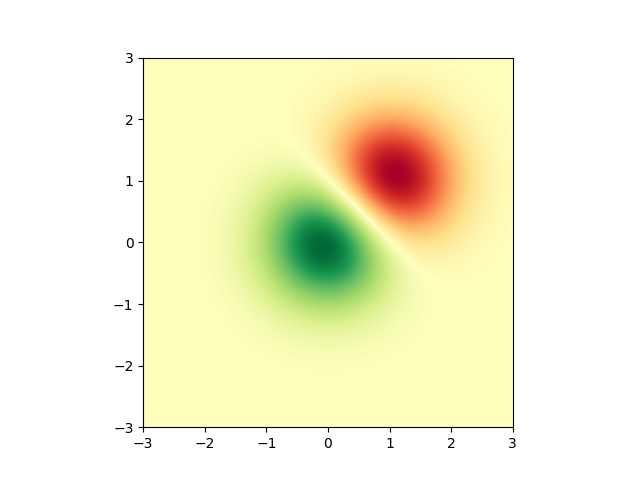
首先，我們將產生一個簡單的二元常態分佈。

delta = 0.025
x = y = np.arange(-3.0, 3.0, delta)
X, Y = np.meshgrid(x, y)
Z1 = np.exp(-X**2 - Y**2)
Z2 = np.exp(-(X - 1)**2 - (Y - 1)**2)
Z = (Z1 - Z2) * 2

fig, ax = plt.subplots()
im = ax.imshow(Z, interpolation='bilinear', cmap=cm.RdYlGn,
               origin='lower', extent=[-3, 3, -3, 3],
               vmax=abs(Z).max(), vmin=-abs(Z).max())

plt.show()

也可以顯示圖片的影像。

# A sample image
with cbook.get_sample_data('grace_hopper.jpg') as image_file:
    image = plt.imread(image_file)

# And another image, using 256x256 16-bit integers.
w, h = 256, 256
with cbook.get_sample_data('s1045.ima.gz') as datafile:
    s = datafile.read()
A = np.frombuffer(s, np.uint16).astype(float).reshape((w, h))
extent = (0, 25, 0, 25)

fig, ax = plt.subplot_mosaic([
    ['hopper', 'mri']
], figsize=(7, 3.5))

ax['hopper'].imshow(image)
ax['hopper'].axis('off')  # clear x-axis and y-axis

im = ax['mri'].imshow(A, cmap=plt.cm.hot, origin='upper', extent=extent)

markers = [(15.9, 14.5), (16.8, 15)]
x, y = zip(*markers)
ax['mri'].plot(x, y, 'o')

ax['mri'].set_title('MRI')

plt.show()

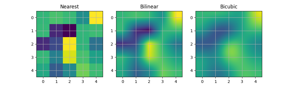
內插影像

也可以在顯示影像之前內插影像。請小心，因為這可能會操縱資料的外觀，但它有助於達到您想要的外觀。以下我們將顯示使用三種不同內插方法內插的相同（小）陣列。

A[i, j] 處像素的中心繪製在 (i+0.5, i+0.5)。如果您使用 interpolation='nearest'，則由 (i, j) 和 (i+1, j+1) 界定的區域將具有相同的顏色。如果您使用內插，則像素中心將具有與最鄰近像素相同的顏色，但其他像素將在相鄰像素之間內插。

為了防止在進行內插時出現邊緣效應，Matplotlib 會在邊緣周圍用相同的像素填充輸入陣列：如果您有一個 5x5 陣列，其中顏色如下所示，a-y

a b c d e
f g h i j
k l m n o
p q r s t
u v w x y

Matplotlib 會在填充陣列上計算內插和調整大小

a a b c d e e
a a b c d e e
f f g h i j j
k k l m n o o
p p q r s t t
o u v w x y y
o u v w x y y

然後擷取結果的中心區域。（極舊版本的 Matplotlib (<0.63) 不會填充陣列，而是調整視圖限制以隱藏受影響的邊緣區域。）

這種方法允許繪製陣列的完整範圍而沒有邊緣效應，例如以不同的內插方法將多個不同大小的影像分層在彼此之上 - 請參閱使用 alpha 混合分層影像。它也意味著效能損失，因為必須建立這個新的臨時填充陣列。複雜的內插也意味著效能損失；為了獲得最大效能或非常大的影像，建議使用 interpolation='nearest'。

A = np.random.rand(5, 5)

fig, axs = plt.subplots(1, 3, figsize=(10, 3))
for ax, interp in zip(axs, ['nearest', 'bilinear', 'bicubic']):
    ax.imshow(A, interpolation=interp)
    ax.set_title(interp.capitalize())
    ax.grid(True)

plt.show()

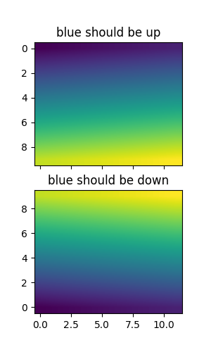
您可以透過使用 origin 參數，指定是否應使用陣列原點 x[0, 0] 在左上角或右下角繪製影像。您也可以在您的 matplotlibrc 檔案中控制預設設定 image.origin。如需有關此主題的更多資訊，請參閱有關原點和範圍的完整指南。

x = np.arange(120).reshape((10, 12))

interp = 'bilinear'
fig, axs = plt.subplots(nrows=2, sharex=True, figsize=(3, 5))
axs[0].set_title('blue should be up')
axs[0].imshow(x, origin='upper', interpolation=interp)

axs[1].set_title('blue should be down')
axs[1].imshow(x, origin='lower', interpolation=interp)
plt.show()

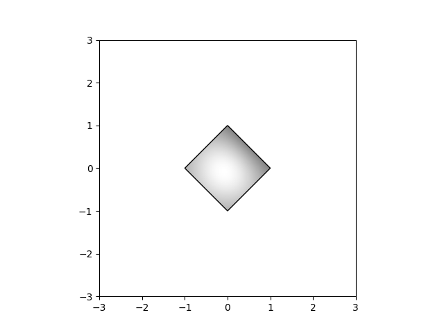
最後，我們將使用剪輯路徑顯示影像。

delta = 0.025
x = y = np.arange(-3.0, 3.0, delta)
X, Y = np.meshgrid(x, y)
Z1 = np.exp(-X**2 - Y**2)
Z2 = np.exp(-(X - 1)**2 - (Y - 1)**2)
Z = (Z1 - Z2) * 2

path = Path([[0, 1], [1, 0], [0, -1], [-1, 0], [0, 1]])
patch = PathPatch(path, facecolor='none')

fig, ax = plt.subplots()
ax.add_patch(patch)

im = ax.imshow(Z, interpolation='bilinear', cmap=cm.gray,
               origin='lower', extent=[-3, 3, -3, 3],
               clip_path=patch, clip_on=True)
im.set_clip_path(patch)

plt.show()

參考

此範例中顯示了以下函式、方法、類別和模組的使用

• matplotlib.axes.Axes.imshow / matplotlib.pyplot.imshow

• matplotlib.artist.Artist.set_clip_path

• matplotlib.patches.PathPatch