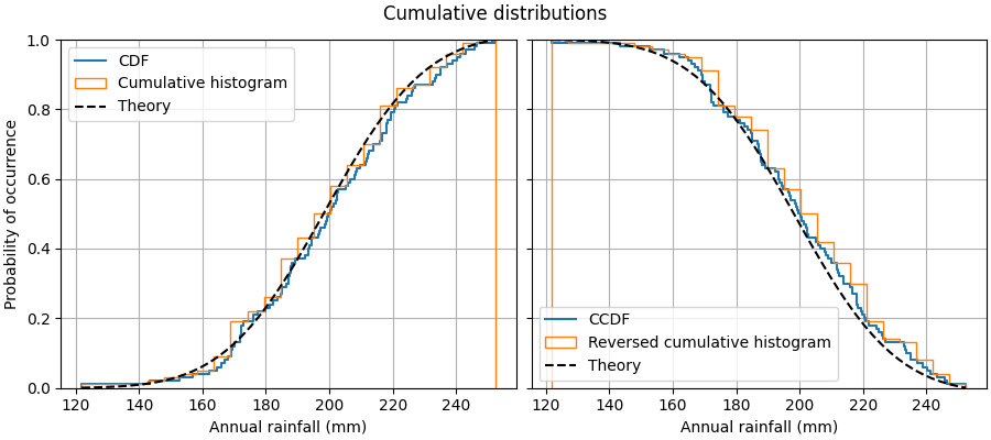
累積分佈#

此範例顯示如何繪製樣本的經驗累積分佈函數 (ECDF)。我們也顯示理論 CDF。

在工程中，ECDF 有時稱為「不超過」曲線：給定 x 值的 y 值表示樣本中觀測值低於該 x 值的機率。例如，x 軸上的值 220 對應於 y 軸上的約 0.80，因此樣本中的觀測值不超過 220 的機率為 80%。相反地，經驗互補累積分佈函數（ECCDF 或「超過」曲線）顯示樣本中觀測值高於值 x 的機率 y。

繪製 ECDF 的直接方法是 Axes.ecdf。傳遞 complementary=True 會產生 ECCDF。

或者，可以使用 ax.hist(data, density=True, cumulative=True) 先將資料分箱，如同繪製直方圖一樣，然後計算並繪製每個分箱中項目頻率的累積總和。在這裡，若要繪製 ECCDF，請傳遞 cumulative=-1。請注意，此方法會產生 E(C)CDF 的近似值，而 Axes.ecdf 是精確的。

import matplotlib.pyplot as plt
import numpy as np

np.random.seed(19680801)

mu = 200
sigma = 25
n_bins = 25
data = np.random.normal(mu, sigma, size=100)

fig = plt.figure(figsize=(9, 4), layout="constrained")
axs = fig.subplots(1, 2, sharex=True, sharey=True)

# Cumulative distributions.
axs[0].ecdf(data, label="CDF")
n, bins, patches = axs[0].hist(data, n_bins, density=True, histtype="step",
                               cumulative=True, label="Cumulative histogram")
x = np.linspace(data.min(), data.max())
y = ((1 / (np.sqrt(2 * np.pi) * sigma)) *
     np.exp(-0.5 * (1 / sigma * (x - mu))**2))
y = y.cumsum()
y /= y[-1]
axs[0].plot(x, y, "k--", linewidth=1.5, label="Theory")

# Complementary cumulative distributions.
axs[1].ecdf(data, complementary=True, label="CCDF")
axs[1].hist(data, bins=bins, density=True, histtype="step", cumulative=-1,
            label="Reversed cumulative histogram")
axs[1].plot(x, 1 - y, "k--", linewidth=1.5, label="Theory")

# Label the figure.
fig.suptitle("Cumulative distributions")
for ax in axs:
    ax.grid(True)
    ax.legend()
    ax.set_xlabel("Annual rainfall (mm)")
    ax.set_ylabel("Probability of occurrence")
    ax.label_outer()

plt.show()

標籤：plot-type: ecdf plot-type: histogram domain: statistics

參考文獻

本範例中顯示下列函數、方法、類別和模組的使用

腳本的總執行時間：（0 分鐘 1.604 秒）

由 Sphinx-Gallery 產生的圖庫