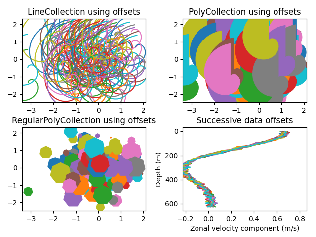
帶自動縮放的線條、多邊形和正多邊形集合#

對於前兩個子圖，我們將使用螺旋。它們的大小將以繪圖單位（而非資料單位）設定。它們的位置將透過 LineCollection 和 PolyCollection 的 offsets 和 offset_transform 關鍵字引數，以資料單位設定。

第三個子圖將繪製正多邊形，其縮放和定位方式與前兩個子圖相同。

最後一個子圖說明如何使用 offsets=(xo, yo)，也就是單一元組而非元組清單，來產生連續偏移的曲線，偏移量以資料單位表示。此行為僅適用於 LineCollection。

import matplotlib.pyplot as plt
import numpy as np

from matplotlib import collections, transforms

nverts = 50
npts = 100

# Make some spirals
r = np.arange(nverts)
theta = np.linspace(0, 2*np.pi, nverts)
xx = r * np.sin(theta)
yy = r * np.cos(theta)
spiral = np.column_stack([xx, yy])

# Fixing random state for reproducibility
rs = np.random.RandomState(19680801)

# Make some offsets
xyo = rs.randn(npts, 2)

# Make a list of colors cycling through the default series.
colors = plt.rcParams['axes.prop_cycle'].by_key()['color']

fig, ((ax1, ax2), (ax3, ax4)) = plt.subplots(2, 2)
fig.subplots_adjust(top=0.92, left=0.07, right=0.97,
                    hspace=0.3, wspace=0.3)


col = collections.LineCollection(
    [spiral], offsets=xyo, offset_transform=ax1.transData)
trans = fig.dpi_scale_trans + transforms.Affine2D().scale(1.0/72.0)
col.set_transform(trans)  # the points to pixels transform
# Note: the first argument to the collection initializer
# must be a list of sequences of (x, y) tuples; we have only
# one sequence, but we still have to put it in a list.
ax1.add_collection(col, autolim=True)
# autolim=True enables autoscaling.  For collections with
# offsets like this, it is neither efficient nor accurate,
# but it is good enough to generate a plot that you can use
# as a starting point.  If you know beforehand the range of
# x and y that you want to show, it is better to set them
# explicitly, leave out the *autolim* keyword argument (or set it to False),
# and omit the 'ax1.autoscale_view()' call below.

# Make a transform for the line segments such that their size is
# given in points:
col.set_color(colors)

ax1.autoscale_view()  # See comment above, after ax1.add_collection.
ax1.set_title('LineCollection using offsets')


# The same data as above, but fill the curves.
col = collections.PolyCollection(
    [spiral], offsets=xyo, offset_transform=ax2.transData)
trans = transforms.Affine2D().scale(fig.dpi/72.0)
col.set_transform(trans)  # the points to pixels transform
ax2.add_collection(col, autolim=True)
col.set_color(colors)


ax2.autoscale_view()
ax2.set_title('PolyCollection using offsets')

# 7-sided regular polygons

col = collections.RegularPolyCollection(
    7, sizes=np.abs(xx) * 10.0, offsets=xyo, offset_transform=ax3.transData)
trans = transforms.Affine2D().scale(fig.dpi / 72.0)
col.set_transform(trans)  # the points to pixels transform
ax3.add_collection(col, autolim=True)
col.set_color(colors)
ax3.autoscale_view()
ax3.set_title('RegularPolyCollection using offsets')


# Simulate a series of ocean current profiles, successively
# offset by 0.1 m/s so that they form what is sometimes called
# a "waterfall" plot or a "stagger" plot.

nverts = 60
ncurves = 20
offs = (0.1, 0.0)

yy = np.linspace(0, 2*np.pi, nverts)
ym = np.max(yy)
xx = (0.2 + (ym - yy) / ym) ** 2 * np.cos(yy - 0.4) * 0.5
segs = []
for i in range(ncurves):
    xxx = xx + 0.02*rs.randn(nverts)
    curve = np.column_stack([xxx, yy * 100])
    segs.append(curve)

col = collections.LineCollection(segs, offsets=offs)
ax4.add_collection(col, autolim=True)
col.set_color(colors)
ax4.autoscale_view()
ax4.set_title('Successive data offsets')
ax4.set_xlabel('Zonal velocity component (m/s)')
ax4.set_ylabel('Depth (m)')
# Reverse the y-axis so depth increases downward
ax4.set_ylim(ax4.get_ylim()[::-1])


plt.show()

LineCollection using offsets, PolyCollection using offsets, RegularPolyCollection using offsets, Successive data offsets

參考文獻

此範例顯示了以下函式、方法、類別和模組的使用

腳本總執行時間： (0 分鐘 1.574 秒)

由 Sphinx-Gallery 產生的圖庫