注意
前往結尾下載完整的範例程式碼。
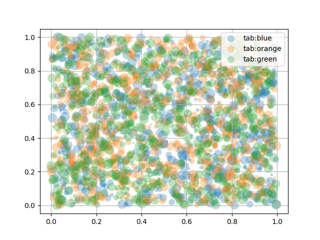
具有圖例的散佈圖#
若要建立具有圖例的散佈圖,可以使用迴圈,並為圖例中顯示的每個項目建立一個 scatter 圖,並相應地設定 label。
以下也示範如何透過在 0 到 1 之間指定 alpha 值來調整標記的透明度。
import matplotlib.pyplot as plt
import numpy as np

np.random.seed(19680801)


fig, ax = plt.subplots()
for color in ['tab:blue', 'tab:orange', 'tab:green']:
    n = 750
    x, y = np.random.rand(2, n)
    scale = 200.0 * np.random.rand(n)
    ax.scatter(x, y, c=color, s=scale, label=color,
               alpha=0.3, edgecolors='none')

ax.legend()
ax.grid(True)

plt.show()
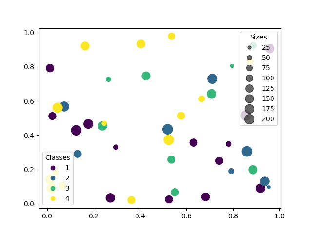
自動圖例建立#
建立散佈圖圖例的另一種方法是使用 PathCollection.legend_elements 方法。它會自動嘗試決定要顯示的有用圖例項目數量,並傳回控制代碼和標籤的元組。這些可以傳遞到對 legend 的呼叫。
N = 45
x, y = np.random.rand(2, N)
c = np.random.randint(1, 5, size=N)
s = np.random.randint(10, 220, size=N)

fig, ax = plt.subplots()

scatter = ax.scatter(x, y, c=c, s=s)

# produce a legend with the unique colors from the scatter
legend1 = ax.legend(*scatter.legend_elements(),
                    loc="lower left", title="Classes")
ax.add_artist(legend1)

# produce a legend with a cross-section of sizes from the scatter
handles, labels = scatter.legend_elements(prop="sizes", alpha=0.6)
legend2 = ax.legend(handles, labels, loc="upper right", title="Sizes")

plt.show()
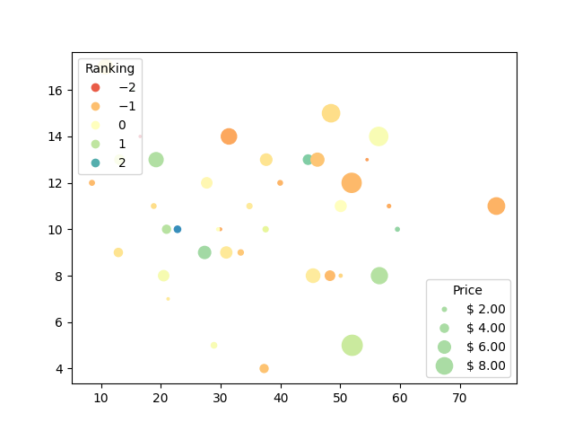
可以將 PathCollection.legend_elements 方法的進一步引數用於控制要建立多少圖例項目以及應如何標記它們。以下展示如何使用它們中的一些。
volume = np.random.rayleigh(27, size=40)
amount = np.random.poisson(10, size=40)
ranking = np.random.normal(size=40)
price = np.random.uniform(1, 10, size=40)

fig, ax = plt.subplots()

# Because the price is much too small when being provided as size for ``s``,
# we normalize it to some useful point sizes, s=0.3*(price*3)**2
scatter = ax.scatter(volume, amount, c=ranking, s=0.3*(price*3)**2,
                     vmin=-3, vmax=3, cmap="Spectral")

# Produce a legend for the ranking (colors). Even though there are 40 different
# rankings, we only want to show 5 of them in the legend.
legend1 = ax.legend(*scatter.legend_elements(num=5),
                    loc="upper left", title="Ranking")
ax.add_artist(legend1)

# Produce a legend for the price (sizes). Because we want to show the prices
# in dollars, we use the *func* argument to supply the inverse of the function
# used to calculate the sizes from above. The *fmt* ensures to show the price
# in dollars. Note how we target at 5 elements here, but obtain only 4 in the
# created legend due to the automatic round prices that are chosen for us.
kw = dict(prop="sizes", num=5, color=scatter.cmap(0.7), fmt="$ {x:.2f}",
          func=lambda s: np.sqrt(s/.3)/3)
legend2 = ax.legend(*scatter.legend_elements(**kw),
                    loc="lower right", title="Price")

plt.show()
參考資料
此範例中顯示了以下函式、方法、類別和模組的使用
指令碼的總執行時間:(0 分鐘 3.632 秒)