注意
前往結尾以下載完整範例程式碼。
Asinh 示範#
說明 asinh 軸刻度,它使用以下轉換
\[a \rightarrow a_0 \sinh^{-1} (a / a_0)\]
對於接近零的座標值(即遠小於「線性寬度」\(a_0\)),這會使數值基本上保持不變
\[a \rightarrow a + \mathcal{O}(a^3)\]
但對於較大的值(即 \(|a| \gg a_0\)),這漸近地等於
\[a \rightarrow a_0 \, \mathrm{sgn}(a) \ln |a| + \mathcal{O}(1)\]
與 symlog 刻度一樣,這允許繪製涵蓋非常寬動態範圍的量,其中包含正值和負值。但是,symlog 包含一個梯度不連續的轉換,因為它是從獨立的線性和對數轉換建構而來。asinh 刻度使用一個對於所有(有限)值都平滑的轉換,這在數學上更簡潔,並減少了與繪圖線性和對數區域之間突然轉換相關的視覺瑕疵。
注意
scale.AsinhScale 是實驗性的,並且 API 可能會變更。
請參閱 AsinhScale, SymmetricalLogScale。
import matplotlib.pyplot as plt
import numpy as np

# Prepare sample values for variations on y=x graph:
x = np.linspace(-3, 6, 500)
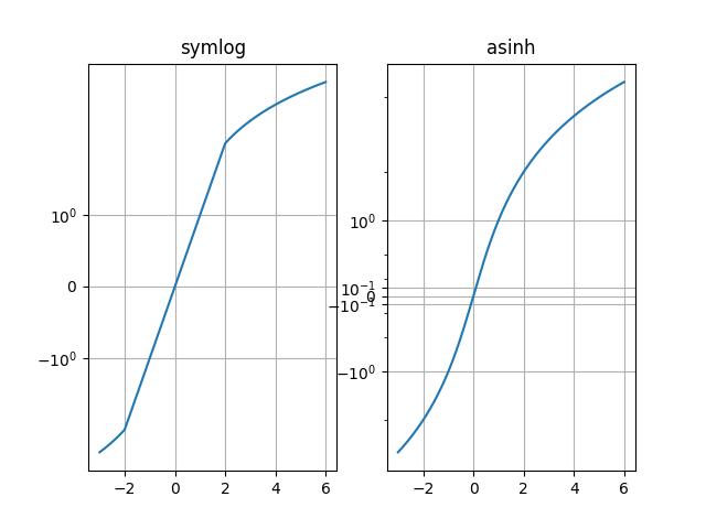
比較 y=x 取樣圖上的「symlog」和「asinh」行為,其中「symlog」在 y=2 附近有不連續的梯度
fig1 = plt.figure()
ax0, ax1 = fig1.subplots(1, 2, sharex=True)

ax0.plot(x, x)
ax0.set_yscale('symlog')
ax0.grid()
ax0.set_title('symlog')

ax1.plot(x, x)
ax1.set_yscale('asinh')
ax1.grid()
ax1.set_title('asinh')
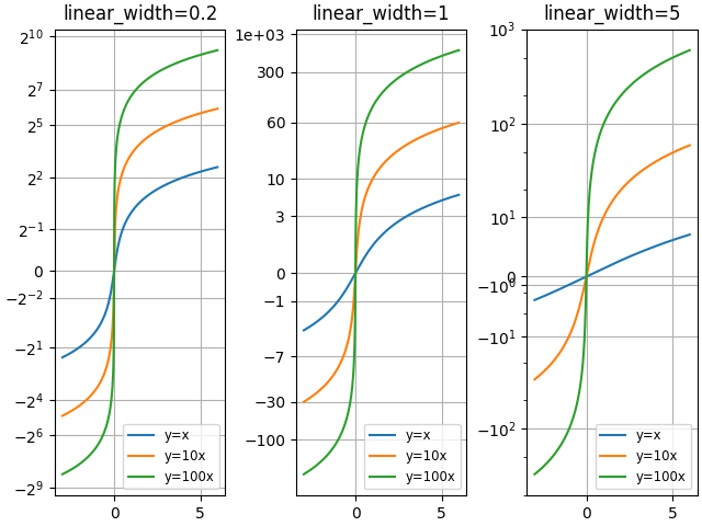
比較具有不同刻度參數「linear_width」的「asinh」圖
fig2 = plt.figure(layout='constrained')
axs = fig2.subplots(1, 3, sharex=True)
for ax, (a0, base) in zip(axs, ((0.2, 2), (1.0, 0), (5.0, 10))):
    ax.set_title(f'linear_width={a0:.3g}')
    ax.plot(x, x, label='y=x')
    ax.plot(x, 10*x, label='y=10x')
    ax.plot(x, 100*x, label='y=100x')
    ax.set_yscale('asinh', linear_width=a0, base=base)
    ax.grid()
    ax.legend(loc='best', fontsize='small')
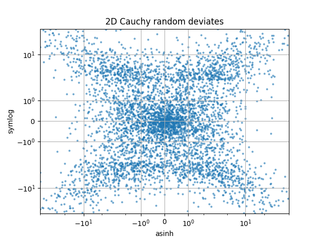
比較 2D 柯西分佈亂數上的「symlog」和「asinh」刻度,其中可能可以在 y=2 附近看到更多由於「symlog」中的梯度不連續性所造成的細微瑕疵
fig3 = plt.figure()
ax = fig3.subplots(1, 1)
r = 3 * np.tan(np.random.uniform(-np.pi / 2.02, np.pi / 2.02,
                                 size=(5000,)))
th = np.random.uniform(0, 2*np.pi, size=r.shape)

ax.scatter(r * np.cos(th), r * np.sin(th), s=4, alpha=0.5)
ax.set_xscale('asinh')
ax.set_yscale('symlog')
ax.set_xlabel('asinh')
ax.set_ylabel('symlog')
ax.set_title('2D Cauchy random deviates')
ax.set_xlim(-50, 50)
ax.set_ylim(-50, 50)
ax.grid()

plt.show()
參考資料
腳本總執行時間: (0 分鐘 2.992 秒)