注意
前往結尾下載完整範例程式碼。
註解#
註解是圖形元素,通常是文字,用於解釋、添加上下文或以其他方式突出顯示視覺化資料的某些部分。annotate 支援多種座標系統,可彈性定位資料和註解彼此之間的相對位置,並提供各種選項來設定文字樣式。Axes.annotate 還提供一個從文字到資料的可選箭頭,並且可以各種方式設定此箭頭的樣式。text 也可用於簡單的文字註解,但它在定位和樣式設定方面不如 annotate 那麼彈性。
基本註解#
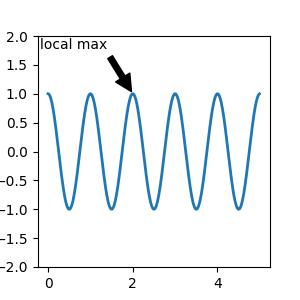
在註解中,有兩點需要考慮:要註解的資料位置 xy 和註解文字的位置 xytext。這兩個參數都是 (x, y) 元組
在此範例中,xy (箭頭尖端) 和 xytext 位置 (文字位置) 都在資料座標中。還有許多其他座標系統可供選擇 -- 您可以使用以下字串之一為 xycoords 和 textcoords 指定 xy 和 xytext 的座標系統 (預設為 'data')
參數 |
座標系統 |
|---|---|
'figure points' |
從圖表的左下角開始的點 |
'figure pixels' |
從圖表的左下角開始的像素 |
'figure fraction' |
(0, 0) 是圖表的左下角,(1, 1) 是右上角 |
'axes points' |
從軸的左下角開始的點 |
'axes pixels' |
從軸的左下角開始的像素 |
'axes fraction' |
(0, 0) 是軸的左下角,(1, 1) 是右上角 |
'data' |
使用軸資料座標系統 |
以下字串也是 textcoords 的有效參數
參數 |
座標系統 |
|---|---|
'offset points' |
從 xy 值偏移 (以點為單位) |
'offset pixels' |
從 xy 值偏移 (以像素為單位) |
對於物理座標系統 (點或像素),原點是圖表或軸的左下角。點是排版點,表示它們是測量 1/72 英寸的物理單位。有關點和像素的更多詳細資訊,請參閱以物理座標繪圖。
註解資料#
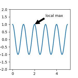
此範例將文字座標放置在軸分數座標中
fig, ax = plt.subplots(figsize=(3, 3))

t = np.arange(0.0, 5.0, 0.01)
s = np.cos(2*np.pi*t)
line, = ax.plot(t, s, lw=2)

ax.annotate('local max', xy=(2, 1), xycoords='data',
            xytext=(0.01, .99), textcoords='axes fraction',
            va='top', ha='left',
            arrowprops=dict(facecolor='black', shrink=0.05))
ax.set_ylim(-2, 2)
註解藝術家#
註解可以相對於 Artist 實例定位,方法是將該藝術家作為 xycoords 傳入。然後,xy 會被解釋為藝術家邊界框的分數。
import matplotlib.patches as mpatches

fig, ax = plt.subplots(figsize=(3, 3))
arr = mpatches.FancyArrowPatch((1.25, 1.5), (1.75, 1.5),
                               arrowstyle='->,head_width=.15', mutation_scale=20)
ax.add_patch(arr)
ax.annotate("label", (.5, .5), xycoords=arr, ha='center', va='bottom')
ax.set(xlim=(1, 2), ylim=(1, 2))
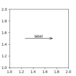
這裡的註解放置在相對於箭頭左下角的位置 (.5, .5),並且在該位置垂直和水平對齊。在垂直方向上,底部會與該參考點對齊,使標籤位於線條上方。有關鏈結註解藝術家的範例,請參閱註解座標系統的藝術家章節。
使用箭頭註解#
您可以通過在可選關鍵字引數 arrowprops 中提供箭頭屬性的字典來啟用從文字到註解點的箭頭繪製。
arrowprops 鍵 |
描述 |
|---|---|
width |
箭頭的寬度 (以點為單位) |
frac |
頭部佔據的箭頭長度比例 |
headwidth |
箭頭頭部底部的寬度 (以點為單位) |
shrink |
將尖端和底部從註解點和文字移動一定百分比 |
**kwargs |
|
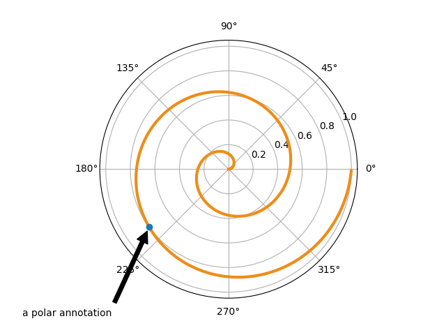
在下面的範例中,xy 點位於資料座標系統中,因為 xycoords 預設為 'data'。對於極座標軸,這是在 (theta, radius) 空間中。在此範例中,文字放置在分數圖表座標系統中。matplotlib.text.Text 關鍵字引數 (例如 horizontalalignment、verticalalignment 和 fontsize) 從 annotate 傳遞到 Text 實例。
fig = plt.figure()
ax = fig.add_subplot(projection='polar')
r = np.arange(0, 1, 0.001)
theta = 2 * 2*np.pi * r
line, = ax.plot(theta, r, color='#ee8d18', lw=3)

ind = 800
thisr, thistheta = r[ind], theta[ind]
ax.plot([thistheta], [thisr], 'o')
ax.annotate('a polar annotation',
            xy=(thistheta, thisr),  # theta, radius
            xytext=(0.05, 0.05),    # fraction, fraction
            textcoords='figure fraction',
            arrowprops=dict(facecolor='black', shrink=0.05),
            horizontalalignment='left',
            verticalalignment='bottom')
有關使用箭頭繪圖的更多資訊,請參閱自訂註解箭頭
相對於資料放置文字註解#
通過將 textcoords 關鍵字引數設定為 'offset points' 或 'offset pixels',可以將註解放置在相對於註解的 xy 輸入的偏移量處。
fig, ax = plt.subplots(figsize=(3, 3))
x = [1, 3, 5, 7, 9]
y = [2, 4, 6, 8, 10]
annotations = ["A", "B", "C", "D", "E"]
ax.scatter(x, y, s=20)

for xi, yi, text in zip(x, y, annotations):
    ax.annotate(text,
                xy=(xi, yi), xycoords='data',
                xytext=(1.5, 1.5), textcoords='offset points')
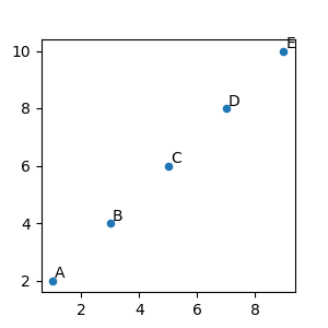
註解會從 xy 值偏移 1.5 點 (1.5*1/72 英寸)。
進階註解#
我們建議您在閱讀本節之前,先閱讀基本註解、text() 和 annotate()。
使用帶框文字註解#
text 接受一個 bbox 關鍵字引數,該引數會在文字周圍繪製一個方框
fig, ax = plt.subplots(figsize=(5, 5))
t = ax.text(0.5, 0.5, "Direction",
            ha="center", va="center", rotation=45, size=15,
            bbox=dict(boxstyle="rarrow,pad=0.3",
                      fc="lightblue", ec="steelblue", lw=2))
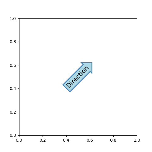
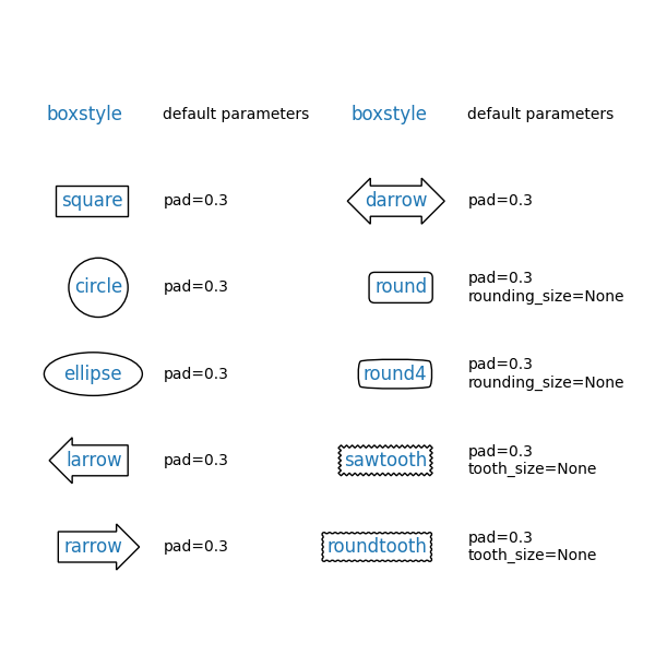
引數是方框樣式的名稱,以及其屬性作為關鍵字引數。目前已實作以下方框樣式
類別 |
名稱 |
屬性 |
|---|---|---|
圓形 |
|
pad=0.3 |
D箭頭 |
|
pad=0.3 |
橢圓形 |
|
pad=0.3 |
L箭頭 |
|
pad=0.3 |
R箭頭 |
|
pad=0.3 |
圓角 |
|
pad=0.3,rounding_size=None |
圓角4 |
|
pad=0.3,rounding_size=None |
圓齒 |
|
pad=0.3,tooth_size=None |
鋸齒 |
|
pad=0.3,tooth_size=None |
方形 |
|
pad=0.3 |
可以使用以下方式存取與文字相關聯的圖塊物件 (方框)
bb = t.get_bbox_patch()
返回值是一個 FancyBboxPatch;圖塊屬性 (facecolor、edgewidth 等) 可以像平常一樣存取和修改。FancyBboxPatch.set_boxstyle 設定方框形狀
bb.set_boxstyle("rarrow", pad=0.6)
屬性引數也可以在樣式名稱中指定,並以逗號分隔
bb.set_boxstyle("rarrow, pad=0.6")
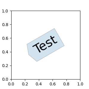
定義自訂方框樣式#
自訂方框樣式可以實作為一個函式,該函式接受指定矩形方框和「變形」量的引數,並傳回「變形」路徑。具體簽名是下面 custom_box_style 的簽名。
在這裡,我們傳回一個新的路徑,該路徑在方框的左側新增一個「箭頭」形狀。
然後,可以透過將 bbox=dict(boxstyle=custom_box_style, ...) 傳遞給 Axes.text 來使用自訂方框樣式。
from matplotlib.path import Path


def custom_box_style(x0, y0, width, height, mutation_size):
    """
    Given the location and size of the box, return the path of the box around it.

    Rotation is automatically taken care of.

    Parameters
    ----------
    x0, y0, width, height : float
       Box location and size.
    mutation_size : float
        Mutation reference scale, typically the text font size.
    """
    # padding
    mypad = 0.3
    pad = mutation_size * mypad
    # width and height with padding added.
    width = width + 2 * pad
    height = height + 2 * pad
    # boundary of the padded box
    x0, y0 = x0 - pad, y0 - pad
    x1, y1 = x0 + width, y0 + height
    # return the new path
    return Path([(x0, y0), (x1, y0), (x1, y1), (x0, y1),
                 (x0-pad, (y0+y1)/2), (x0, y0), (x0, y0)],
                closed=True)

fig, ax = plt.subplots(figsize=(3, 3))
ax.text(0.5, 0.5, "Test", size=30, va="center", ha="center", rotation=30,
        bbox=dict(boxstyle=custom_box_style, alpha=0.2))
同樣地,自訂方框樣式可以實作為實作 __call__ 的類別。
然後,可以將這些類別註冊到 BoxStyle._style_list 字典中,這允許將方框樣式指定為字串,bbox=dict(boxstyle="registered_name,param=value,...", ...)。請注意,此註冊依賴內部 API,因此並非正式支援。
from matplotlib.patches import BoxStyle


class MyStyle:
    """A simple box."""

    def __init__(self, pad=0.3):
        """
        The arguments must be floats and have default values.

        Parameters
        ----------
        pad : float
            amount of padding
        """
        self.pad = pad
        super().__init__()

    def __call__(self, x0, y0, width, height, mutation_size):
        """
        Given the location and size of the box, return the path of the box around it.

        Rotation is automatically taken care of.

        Parameters
        ----------
        x0, y0, width, height : float
            Box location and size.
        mutation_size : float
            Reference scale for the mutation, typically the text font size.
        """
        # padding
        pad = mutation_size * self.pad
        # width and height with padding added
        width = width + 2 * pad
        height = height + 2 * pad
        # boundary of the padded box
        x0, y0 = x0 - pad, y0 - pad
        x1, y1 = x0 + width, y0 + height
        # return the new path
        return Path([(x0, y0), (x1, y0), (x1, y1), (x0, y1),
                     (x0-pad, (y0+y1)/2), (x0, y0), (x0, y0)],
                    closed=True)


BoxStyle._style_list["angled"] = MyStyle  # Register the custom style.

fig, ax = plt.subplots(figsize=(3, 3))
ax.text(0.5, 0.5, "Test", size=30, va="center", ha="center", rotation=30,
        bbox=dict(boxstyle="angled,pad=0.5", alpha=0.2))

del BoxStyle._style_list["angled"]  # Unregister it.
同樣地,您可以定義自訂 ConnectionStyle 和自訂 ArrowStyle。請檢視 patches 的原始碼,以瞭解每個類別的定義方式。
自訂註解箭頭#
可以透過指定 arrowprops 引數來選擇性地繪製將 xy 連接到 xytext 的箭頭。若要僅繪製箭頭,請使用空字串作為第一個引數
fig, ax = plt.subplots(figsize=(3, 3))
ax.annotate("",
            xy=(0.2, 0.2), xycoords='data',
            xytext=(0.8, 0.8), textcoords='data',
            arrowprops=dict(arrowstyle="->", connectionstyle="arc3"))
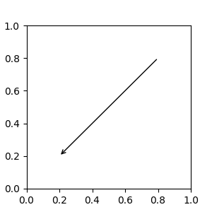
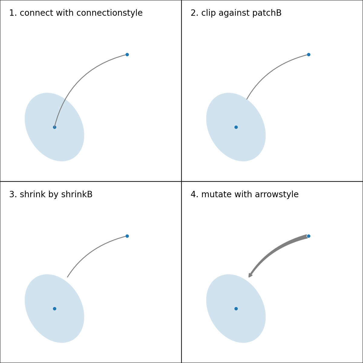
箭頭繪製如下
建立連接兩點的路徑,如 connectionstyle 參數所指定。
若已設定,則會剪裁路徑以避免圖塊 patchA 和 patchB。
路徑會進一步縮小 shrinkA 和 shrinkB (以像素為單位)。
路徑會根據 arrowstyle 參數的指定,變形為箭頭圖塊。
兩點之間的連接路徑建立是由 connectionstyle 鍵控制,並且提供下列樣式
名稱 |
屬性 |
|---|---|
|
angleA=90,angleB=0,rad=0.0 |
|
angleA=90,angleB=0 |
|
angleA=0,angleB=0,armA=None,armB=None,rad=0.0 |
|
rad=0.0 |
|
armA=0.0,armB=0.0,fraction=0.3,angle=None |
請注意,angle3 和 arc3 中的「3」表示結果路徑是二次樣條曲線段 (三個控制點)。如下所述,某些箭頭樣式選項只能在連接路徑是二次樣條曲線時使用。
以下範例 (有限地) 示範了每個連接樣式的行為。(警告:bar 樣式的行為目前未明確定義,且未來可能會變更)。
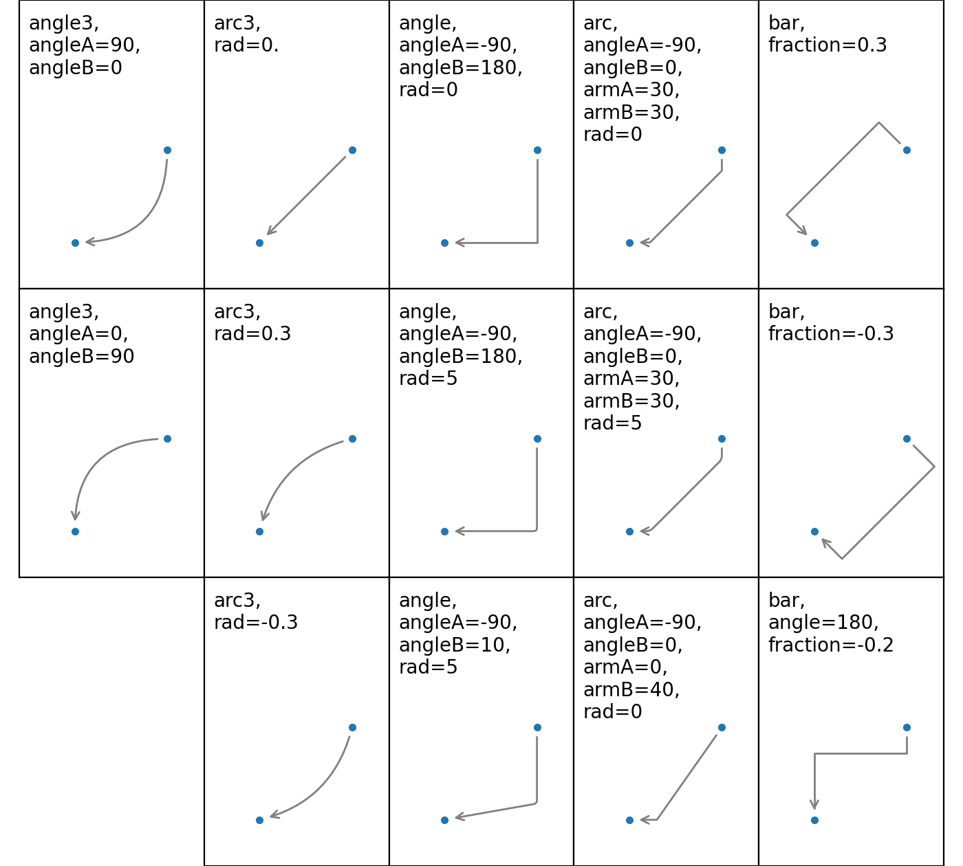
註解的連接樣式
然後,根據給定的 arrowstyle,將連接路徑 (在剪裁和縮小之後) 變形為箭頭圖塊
名稱 |
屬性 |
|---|---|
|
無 |
|
head_length=0.4,head_width=0.2 |
|
widthB=1.0,lengthB=0.2,angleB=None |
|
widthA=1.0,widthB=1.0 |
|
head_length=0.4,head_width=0.2 |
|
head_length=0.4,head_width=0.2 |
|
head_length=0.4,head_width=0.2 |
|
head_length=0.4,head_width=0.2 |
|
head_length=0.4,head_width=0.2 |
|
head_length=0.4,head_width=0.4,tail_width=0.4 |
|
head_length=0.5,head_width=0.5,tail_width=0.2 |
|
tail_width=0.3,shrink_factor=0.5 |
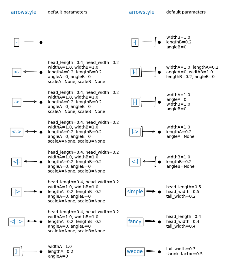
某些箭頭樣式僅適用於產生二次樣條曲線段的連接樣式。它們是 fancy、simple 和 wedge。對於這些箭頭樣式,您必須使用「angle3」或「arc3」連接樣式。
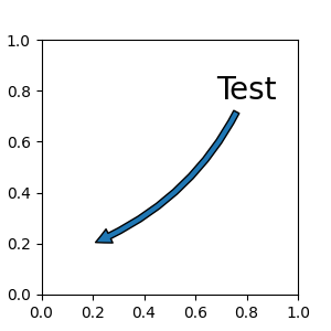
如果提供註解字串,則預設會將圖塊設定為文字的 bbox 圖塊。
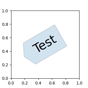
fig, ax = plt.subplots(figsize=(3, 3))

ax.annotate("Test",
            xy=(0.2, 0.2), xycoords='data',
            xytext=(0.8, 0.8), textcoords='data',
            size=20, va="center", ha="center",
            arrowprops=dict(arrowstyle="simple",
                            connectionstyle="arc3,rad=-0.2"))
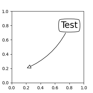
如同 text,可以使用 bbox 引數在文字周圍繪製方框。
fig, ax = plt.subplots(figsize=(3, 3))

ann = ax.annotate("Test",
                  xy=(0.2, 0.2), xycoords='data',
                  xytext=(0.8, 0.8), textcoords='data',
                  size=20, va="center", ha="center",
                  bbox=dict(boxstyle="round4", fc="w"),
                  arrowprops=dict(arrowstyle="-|>",
                                  connectionstyle="arc3,rad=-0.2",
                                  fc="w"))
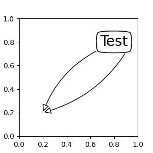
預設情況下,起點設定為文字範圍的中心。可以使用 relpos 鍵值來調整。這些值會標準化為文字的範圍。例如,(0, 0) 表示左下角,而 (1, 1) 表示右上角。
fig, ax = plt.subplots(figsize=(3, 3))

ann = ax.annotate("Test",
                  xy=(0.2, 0.2), xycoords='data',
                  xytext=(0.8, 0.8), textcoords='data',
                  size=20, va="center", ha="center",
                  bbox=dict(boxstyle="round4", fc="w"),
                  arrowprops=dict(arrowstyle="-|>",
                                  connectionstyle="arc3,rad=0.2",
                                  relpos=(0., 0.),
                                  fc="w"))

ann = ax.annotate("Test",
                  xy=(0.2, 0.2), xycoords='data',
                  xytext=(0.8, 0.8), textcoords='data',
                  size=20, va="center", ha="center",
                  bbox=dict(boxstyle="round4", fc="w"),
                  arrowprops=dict(arrowstyle="-|>",
                                  connectionstyle="arc3,rad=-0.2",
                                  relpos=(1., 0.),
                                  fc="w"))
將藝術家放置在錨定軸位置#
有一些藝術家類別可以放置在軸中的錨定位置。常見的範例是圖例。可以使用 OffsetBox 類別建立此類型的藝術家。matplotlib.offsetbox 和 mpl_toolkits.axes_grid1.anchored_artists 中提供一些預先定義的類別。
from matplotlib.offsetbox import AnchoredText

fig, ax = plt.subplots(figsize=(3, 3))
at = AnchoredText("Figure 1a",
                  prop=dict(size=15), frameon=True, loc='upper left')
at.patch.set_boxstyle("round,pad=0.,rounding_size=0.2")
ax.add_artist(at)
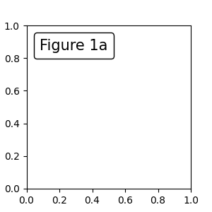
loc 關鍵字的含義與圖例命令中的含義相同。
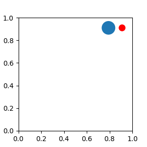
一個簡單的應用是,當藝術家 (或藝術家集合) 的大小在建立時以像素大小已知時。例如,如果您要繪製一個固定大小為 20 像素 x 20 像素 (半徑 = 10 像素) 的圓形,則可以使用 AnchoredDrawingArea。該執行個體是使用繪圖區域的大小 (以像素為單位) 建立的,並且可以在繪圖區域中新增任意藝術家。請注意,新增至繪圖區域的藝術家範圍與繪圖區域本身的放置無關。只有初始大小重要。
新增至繪圖區域的藝術家不應設定轉換 (它將被覆寫),並且這些藝術家的尺寸會被解譯為像素座標,也就是說,上例中圓形的半徑分別為 10 像素和 5 像素。
from matplotlib.patches import Circle
from mpl_toolkits.axes_grid1.anchored_artists import AnchoredDrawingArea

fig, ax = plt.subplots(figsize=(3, 3))
ada = AnchoredDrawingArea(40, 20, 0, 0,
                          loc='upper right', pad=0., frameon=False)
p1 = Circle((10, 10), 10)
ada.drawing_area.add_artist(p1)
p2 = Circle((30, 10), 5, fc="r")
ada.drawing_area.add_artist(p2)
ax.add_artist(ada)
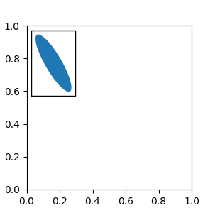
有時,您希望藝術家能夠隨著資料座標 (或畫布像素以外的座標) 縮放。您可以使用 AnchoredAuxTransformBox 類別。這與 AnchoredDrawingArea 類似,不同之處在於藝術家的範圍是在繪圖期間根據指定的轉換來判斷。
以下範例中的橢圓形將具有對應於資料座標中 0.1 和 0.4 的寬度和高度,並且當軸的檢視限制變更時,將會自動縮放。
from matplotlib.patches import Ellipse
from mpl_toolkits.axes_grid1.anchored_artists import AnchoredAuxTransformBox

fig, ax = plt.subplots(figsize=(3, 3))
box = AnchoredAuxTransformBox(ax.transData, loc='upper left')
el = Ellipse((0, 0), width=0.1, height=0.4, angle=30)  # in data coordinates!
box.drawing_area.add_artist(el)
ax.add_artist(box)
另一種相對於父 Axes 或錨點固定藝術家 (artist) 的方法是透過 AnchoredOffsetbox 的 bbox_to_anchor 參數。然後,可以使用 HPacker 和 VPacker 將此藝術家自動定位於另一個藝術家。
from matplotlib.offsetbox import (AnchoredOffsetbox, DrawingArea, HPacker,
                                  TextArea)

fig, ax = plt.subplots(figsize=(3, 3))

box1 = TextArea(" Test: ", textprops=dict(color="k"))
box2 = DrawingArea(60, 20, 0, 0)

el1 = Ellipse((10, 10), width=16, height=5, angle=30, fc="r")
el2 = Ellipse((30, 10), width=16, height=5, angle=170, fc="g")
el3 = Ellipse((50, 10), width=16, height=5, angle=230, fc="b")
box2.add_artist(el1)
box2.add_artist(el2)
box2.add_artist(el3)

box = HPacker(children=[box1, box2],
              align="center",
              pad=0, sep=5)

anchored_box = AnchoredOffsetbox(loc='lower left',
                                 child=box, pad=0.,
                                 frameon=True,
                                 bbox_to_anchor=(0., 1.02),
                                 bbox_transform=ax.transAxes,
                                 borderpad=0.,)

ax.add_artist(anchored_box)
fig.subplots_adjust(top=0.8)
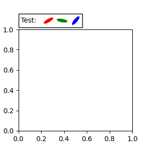
請注意,與 Legend 不同,預設情況下,bbox_transform 會設為 IdentityTransform。
註解的座標系統#
Matplotlib 註解支援多種類型的座標系統。在 基本註解 中的範例使用了 data 座標系統;其他一些更進階的選項如下:
Transform 實例#
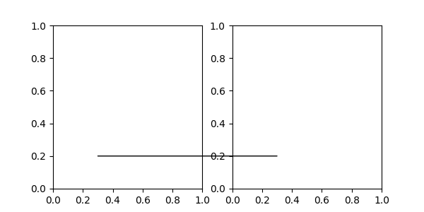
Transforms 將座標映射到不同的座標系統,通常是顯示座標系統。有關詳細說明,請參閱 轉換教學。在此,Transform 物件用於識別對應點的座標系統。例如,Axes.transAxes 轉換將註解定位於相對於 Axes 座標的位置;因此,使用它等同於將座標系統設為「axes 分數」。
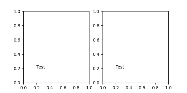
fig, (ax1, ax2) = plt.subplots(nrows=1, ncols=2, figsize=(6, 3))
ax1.annotate("Test", xy=(0.2, 0.2), xycoords=ax1.transAxes)
ax2.annotate("Test", xy=(0.2, 0.2), xycoords="axes fraction")
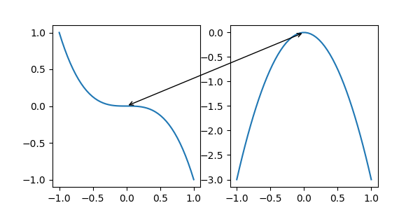
另一個常用的 Transform 實例是 Axes.transData。此轉換是繪製在 Axes 中的資料的座標系統。在此範例中,它用於在兩個 Axes 中的相關資料點之間繪製箭頭。我們傳遞了空白文字,因為在這種情況下,註解會連接資料點。
x = np.linspace(-1, 1)

fig, (ax1, ax2) = plt.subplots(nrows=1, ncols=2, figsize=(6, 3))
ax1.plot(x, -x**3)
ax2.plot(x, -3*x**2)
ax2.annotate("",
             xy=(0, 0), xycoords=ax1.transData,
             xytext=(0, 0), textcoords=ax2.transData,
             arrowprops=dict(arrowstyle="<->"))
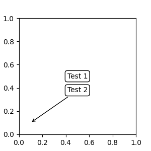
Artist 實例#
xy 值(或 xytext)會被解釋為藝術家 (artist) 的邊界框 (bbox) 的分數座標。
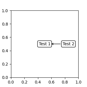
fig, ax = plt.subplots(nrows=1, ncols=1, figsize=(3, 3))
an1 = ax.annotate("Test 1",
                  xy=(0.5, 0.5), xycoords="data",
                  va="center", ha="center",
                  bbox=dict(boxstyle="round", fc="w"))

an2 = ax.annotate("Test 2",
                  xy=(1, 0.5), xycoords=an1,  # (1, 0.5) of an1's bbox
                  xytext=(30, 0), textcoords="offset points",
                  va="center", ha="left",
                  bbox=dict(boxstyle="round", fc="w"),
                  arrowprops=dict(arrowstyle="->"))

請注意,您必須確保在繪製 an2 之前,已確定座標藝術家 (本範例中的 an1) 的範圍。通常,這表示 an2 需要在 an1 之後繪製。所有邊界框的基底類別是 BboxBase。
傳回 Transform 或 BboxBase 的可呼叫物件#
一個可呼叫的物件,它會將渲染器 (renderer) 實例當作單一引數,並傳回 Transform 或 BboxBase。例如,Artist.get_window_extent 的傳回值是一個 bbox,因此此方法與 (2) 傳入藝術家 (artist) 相同。
fig, ax = plt.subplots(nrows=1, ncols=1, figsize=(3, 3))
an1 = ax.annotate("Test 1",
                  xy=(0.5, 0.5), xycoords="data",
                  va="center", ha="center",
                  bbox=dict(boxstyle="round", fc="w"))

an2 = ax.annotate("Test 2",
                  xy=(1, 0.5), xycoords=an1.get_window_extent,
                  xytext=(30, 0), textcoords="offset points",
                  va="center", ha="left",
                  bbox=dict(boxstyle="round", fc="w"),
                  arrowprops=dict(arrowstyle="->"))
Artist.get_window_extent 是 Axes 物件的邊界框,因此與將座標系統設為 axes 分數相同。
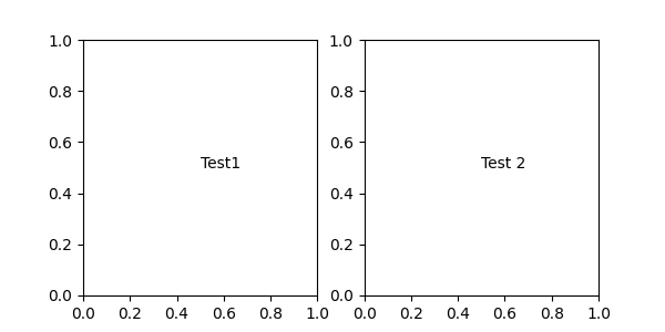
fig, (ax1, ax2) = plt.subplots(nrows=1, ncols=2, figsize=(6, 3))

an1 = ax1.annotate("Test1", xy=(0.5, 0.5), xycoords="axes fraction")
an2 = ax2.annotate("Test 2", xy=(0.5, 0.5), xycoords=ax2.get_window_extent)
混合座標規格#
一對混合的座標規格 -- 第一個用於 x 座標,第二個用於 y 座標。例如,x=0.5 是以資料座標表示,而 y=1 是以標準化的 axes 座標表示。
fig, ax = plt.subplots(figsize=(3, 3))
ax.annotate("Test", xy=(0.5, 1), xycoords=("data", "axes fraction"))
ax.axvline(x=.5, color='lightgray')
ax.set(xlim=(0, 2), ylim=(1, 2))
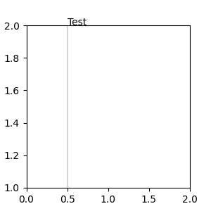
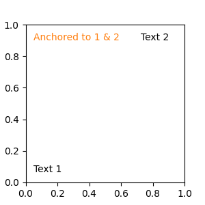
任何支援的座標系統都可以用於混合規格中。例如,文字「Anchored to 1 & 2」是相對於兩個 Text 藝術家 (artist) 定位的。
text.OffsetFrom#
有時,您會希望註解的「偏移點」不是來自被註解的點,而是來自其他點或藝術家 (artist)。text.OffsetFrom 是用於處理此類情況的輔助工具。
from matplotlib.text import OffsetFrom

fig, ax = plt.subplots(figsize=(3, 3))
an1 = ax.annotate("Test 1", xy=(0.5, 0.5), xycoords="data",
                  va="center", ha="center",
                  bbox=dict(boxstyle="round", fc="w"))

offset_from = OffsetFrom(an1, (0.5, 0))
an2 = ax.annotate("Test 2", xy=(0.1, 0.1), xycoords="data",
                  xytext=(0, -10), textcoords=offset_from,
                  # xytext is offset points from "xy=(0.5, 0), xycoords=an1"
                  va="top", ha="center",
                  bbox=dict(boxstyle="round", fc="w"),
                  arrowprops=dict(arrowstyle="->"))
非文字註解#
使用 ConnectionPatch#
ConnectionPatch 就像沒有文字的註解。雖然在大多數情況下 annotate 就已足夠,但當您想要連接不同 Axes 中的點時,ConnectionPatch 會很有用。例如,在這裡,我們將 ax1 的資料座標中的點 xy 連接到 ax2 的資料座標中的點 xy。
from matplotlib.patches import ConnectionPatch

fig, (ax1, ax2) = plt.subplots(nrows=1, ncols=2, figsize=(6, 3))
xy = (0.3, 0.2)
con = ConnectionPatch(xyA=xy, coordsA=ax1.transData,
                      xyB=xy, coordsB=ax2.transData)

fig.add_artist(con)
在這裡,我們將 ConnectionPatch 添加到 figure(使用 add_artist),而不是添加到任一 Axes。這可確保 ConnectionPatch 藝術家 (artist) 繪製在兩個 Axes 的頂部,並且在使用 constrained_layout 定位 Axes 時也是必要的。
Axes 之間的縮放效果#
mpl_toolkits.axes_grid1.inset_locator 定義了一些用於連接兩個 Axes 的有用修補程式類別 (patch class)。
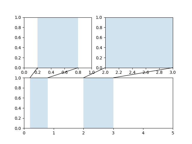
此圖形的程式碼位於 Axes 縮放效果,建議熟悉 轉換教學。
指令碼的總執行時間: (0 分鐘 4.605 秒)