注意

跳到結尾下載完整的範例程式碼。

在圖表中排列多個軸#

通常，我們希望在一個圖表上一次顯示多個軸，通常組織成一個規則的網格。Matplotlib 提供了多種工具來處理軸的網格，這些工具在函式庫的歷史中不斷演進。在這裡，我們將討論我們認為使用者應該最常使用的工具、軸組織方式的基礎工具，並提及一些較舊的工具。

注意

Matplotlib 使用「軸」來指代包含數據、x 軸和 y 軸、刻度、標籤、標題等的繪圖區域。有關更多詳細資訊，請參閱圖表的部分。另一個常用的術語是「子圖」，指的是在網格中與其他軸物件一起的軸。

概述#

建立網格狀的軸組合#

subplots: 用於建立圖表和軸網格的主要函數。它一次在圖表上建立並放置所有軸，並傳回一個物件陣列，其中包含網格中軸的控制代碼。請參閱 Figure.subplots。

或

subplot_mosaic: 建立圖表和軸網格的簡單方法，並增加了軸也可以跨越行或列的靈活性。軸會以標記的字典而不是陣列的形式傳回。另請參閱 Figure.subplot_mosaic 和複雜且語意的圖表組成 (subplot_mosaic)。

有時，自然會有一個以上的不同軸網格群組，在這種情況下，Matplotlib 具有 SubFigure 的概念

SubFigure: 圖表內的虛擬圖表。

底層工具#

這些的基礎是 GridSpec 和 SubplotSpec 的概念

GridSpec: 指定子圖將放置的網格幾何。需要設定網格的列數和欄數。您可以選擇調整子圖佈局參數（例如，左側、右側等）。
SubplotSpec: 指定子圖在給定 GridSpec 中的位置。

一次新增單個軸#

上述函式會在單個函式呼叫中建立所有軸。也可以一次新增一個軸，這原本是 Matplotlib 的運作方式。這樣做通常較不優雅和靈活，但有時對於互動式工作或將軸放置在自訂位置很有用

add_axes: 在圖表寬度或高度的小數部分中，於 [左側, 底部, 寬度, 高度] 指定的位置新增單個軸。
subplot 或 Figure.add_subplot: 在圖表上新增單個子圖，並以 1 為基礎的索引 (從 Matlab 繼承)。透過指定網格單元格的範圍，可以跨越列和行。
subplot2grid: 與 pyplot.subplot 相似，但使用以 0 為基礎的索引和二維 Python 切片來選擇單元格。

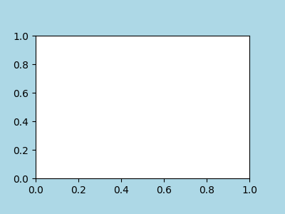
作為手動新增軸 ax 的簡單範例，讓我們將一個 3 英寸 x 2 英寸的軸新增到 4 英寸 x 3 英寸的圖表中。請注意，子圖的位置定義為圖表標準化單位中的 [左側、底部、寬度、高度]

import matplotlib.pyplot as plt
import numpy as np

w, h = 4, 3
margin = 0.5
fig = plt.figure(figsize=(w, h), facecolor='lightblue')
ax = fig.add_axes([margin / w, margin / h, (w - 2 * margin) / w,
                      (h - 2 * margin) / h])

用於建立網格的高階方法#

基本的 2x2 網格#

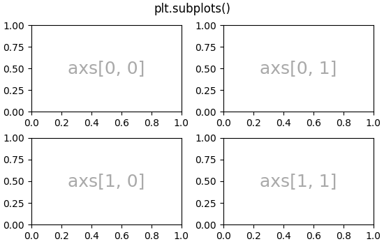
我們可以透過使用 subplots 來建立基本的 2x2 軸網格。它會傳回 Figure 實例和 Axes 物件的陣列。軸物件可以用來存取方法，以在軸上放置藝術家；這裡我們使用 annotate，但其他範例可能是 plot、pcolormesh 等等。

fig, axs = plt.subplots(ncols=2, nrows=2, figsize=(5.5, 3.5),
                        layout="constrained")
# add an artist, in this case a nice label in the middle...
for row in range(2):
    for col in range(2):
        axs[row, col].annotate(f'axs[{row}, {col}]', (0.5, 0.5),
                               transform=axs[row, col].transAxes,
                               ha='center', va='center', fontsize=18,
                               color='darkgrey')
fig.suptitle('plt.subplots()')

我們將註釋許多軸，因此讓我們封裝註釋，而不是每次需要時都使用那麼大段註釋程式碼

def annotate_axes(ax, text, fontsize=18):
    ax.text(0.5, 0.5, text, transform=ax.transAxes,
            ha="center", va="center", fontsize=fontsize, color="darkgrey")

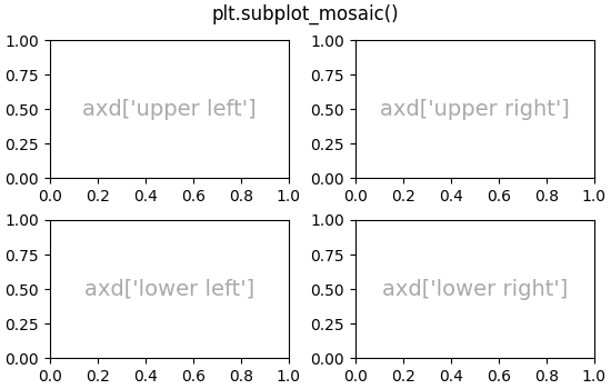
可以使用 subplot_mosaic 達到相同的效果，但傳回類型是字典而不是陣列，使用者可以在其中為鍵提供有用的意義。這裡我們提供兩個列表，每個列表代表一行，並且列表中的每個元素代表一欄的鍵。

fig, axd = plt.subplot_mosaic([['upper left', 'upper right'],
                               ['lower left', 'lower right']],
                              figsize=(5.5, 3.5), layout="constrained")
for k, ax in axd.items():
    annotate_axes(ax, f'axd[{k!r}]', fontsize=14)
fig.suptitle('plt.subplot_mosaic()')

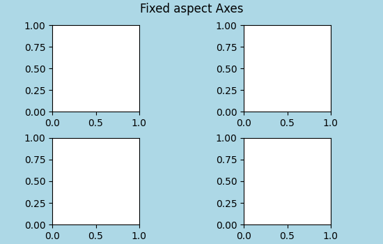
固定長寬比軸的網格#

固定長寬比軸在影像或地圖中很常見。但是，它們對佈局提出了挑戰，因為軸的大小施加了兩組約束 - 它們符合圖表的大小並且具有設定的長寬比。這導致預設情況下軸之間存在很大的間隙

fig, axs = plt.subplots(2, 2, layout="constrained",
                        figsize=(5.5, 3.5), facecolor='lightblue')
for ax in axs.flat:
    ax.set_aspect(1)
fig.suptitle('Fixed aspect Axes')

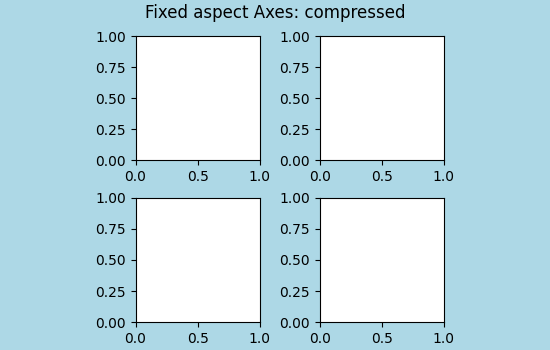
解決此問題的一種方法是將圖表的長寬比變更為接近軸的長寬比，但是這需要反覆試驗。Matplotlib 也提供了 layout="compressed"，它會與簡單的網格一起運作，以減少軸之間的間隙。(mpl_toolkits 也提供 ImageGrid 來達成類似的效果，但使用非標準的軸類別)。

fig, axs = plt.subplots(2, 2, layout="compressed", figsize=(5.5, 3.5),
                        facecolor='lightblue')
for ax in axs.flat:
    ax.set_aspect(1)
fig.suptitle('Fixed aspect Axes: compressed')

跨越網格中行或列的軸#

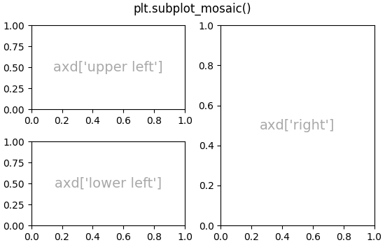
有時我們希望軸跨越網格的行或列。實際上有多種方法可以實現此目的，但最方便的方法可能是透過重複其中一個鍵來使用 subplot_mosaic

fig, axd = plt.subplot_mosaic([['upper left', 'right'],
                               ['lower left', 'right']],
                              figsize=(5.5, 3.5), layout="constrained")
for k, ax in axd.items():
    annotate_axes(ax, f'axd[{k!r}]', fontsize=14)
fig.suptitle('plt.subplot_mosaic()')

請參閱下文，了解如何使用 GridSpec 或 subplot2grid 來執行相同的操作。

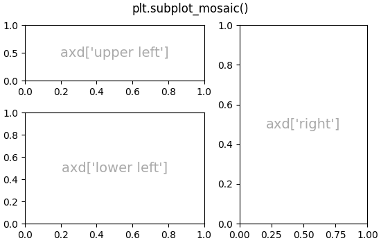
網格中可變的寬度或高度#

subplots 和 subplot_mosaic 都允許使用 gridspec_kw 關鍵字引數，使格線中的列具有不同的高度，且行具有不同的寬度。 GridSpec 接受的間距參數可以傳遞給 subplots 和 subplot_mosaic。

gs_kw = dict(width_ratios=[1.4, 1], height_ratios=[1, 2])
fig, axd = plt.subplot_mosaic([['upper left', 'right'],
                               ['lower left', 'right']],
                              gridspec_kw=gs_kw, figsize=(5.5, 3.5),
                              layout="constrained")
for k, ax in axd.items():
    annotate_axes(ax, f'axd[{k!r}]', fontsize=14)
fig.suptitle('plt.subplot_mosaic()')

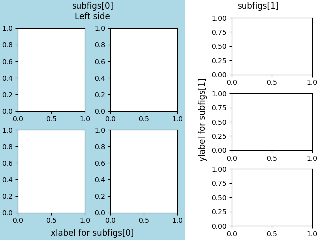
巢狀軸配置#

有時，擁有兩個或多個可能不需要彼此關聯的軸格線會很有幫助。實現此目的最簡單的方法是使用 Figure.subfigures。請注意，子圖配置是獨立的，因此每個子圖中的軸脊柱不一定對齊。請參閱下文，了解使用 GridSpecFromSubplotSpec 達到相同效果的更詳細方法。

fig = plt.figure(layout="constrained")
subfigs = fig.subfigures(1, 2, wspace=0.07, width_ratios=[1.5, 1.])
axs0 = subfigs[0].subplots(2, 2)
subfigs[0].set_facecolor('lightblue')
subfigs[0].suptitle('subfigs[0]\nLeft side')
subfigs[0].supxlabel('xlabel for subfigs[0]')

axs1 = subfigs[1].subplots(3, 1)
subfigs[1].suptitle('subfigs[1]')
subfigs[1].supylabel('ylabel for subfigs[1]')

也可以使用巢狀列表透過 subplot_mosaic 來巢狀化軸。此方法不使用子圖（如上所述），因此無法新增每個子圖的 suptitle 和 supxlabel 等。它只是 subgridspec 方法的便捷包裝器，如下所述。

inner = [['innerA'],
         ['innerB']]
outer = [['upper left',  inner],
          ['lower left', 'lower right']]

fig, axd = plt.subplot_mosaic(outer, layout="constrained")
for k, ax in axd.items():
    annotate_axes(ax, f'axd[{k!r}]')

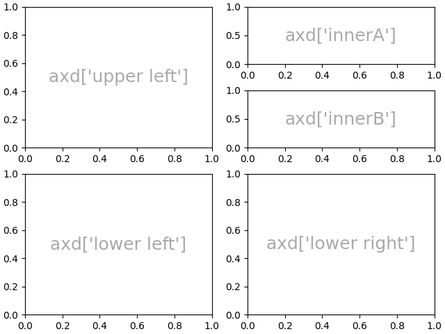
低階和進階格線方法#

在內部，軸格線的排列由建立 GridSpec 和 SubplotSpec 的實例來控制。 GridSpec 定義一個（可能不均勻的）格線單元格。索引到 GridSpec 會傳回涵蓋一個或多個格線單元格的 SubplotSpec，可用於指定軸的位置。

以下範例顯示如何使用低階方法，透過 GridSpec 物件排列軸。

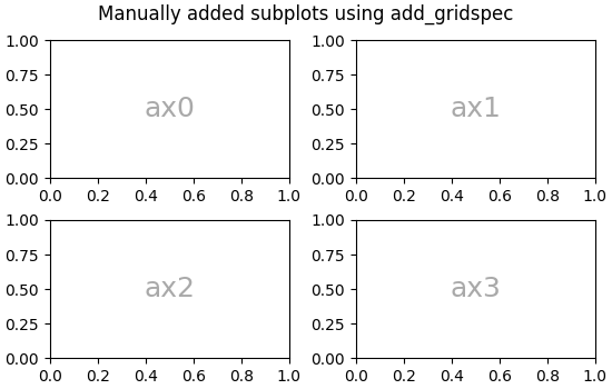
基本 2x2 格線#

我們可以採用與 plt.subplots(2, 2) 相同的方式完成 2x2 格線

fig = plt.figure(figsize=(5.5, 3.5), layout="constrained")
spec = fig.add_gridspec(ncols=2, nrows=2)

ax0 = fig.add_subplot(spec[0, 0])
annotate_axes(ax0, 'ax0')

ax1 = fig.add_subplot(spec[0, 1])
annotate_axes(ax1, 'ax1')

ax2 = fig.add_subplot(spec[1, 0])
annotate_axes(ax2, 'ax2')

ax3 = fig.add_subplot(spec[1, 1])
annotate_axes(ax3, 'ax3')

fig.suptitle('Manually added subplots using add_gridspec')

Manually added subplots using add_gridspec

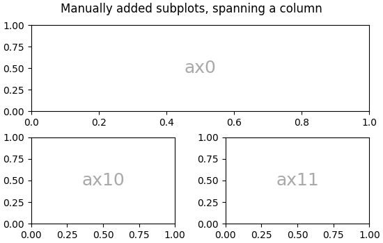
軸跨越格線中的列或格線#

我們可以使用 NumPy 切片語法為 spec 陣列建立索引，而新的軸將跨越該切片。這會與 fig, axd = plt.subplot_mosaic([['ax0', 'ax0'], ['ax1', 'ax2']], ...) 相同

fig = plt.figure(figsize=(5.5, 3.5), layout="constrained")
spec = fig.add_gridspec(2, 2)

ax0 = fig.add_subplot(spec[0, :])
annotate_axes(ax0, 'ax0')

ax10 = fig.add_subplot(spec[1, 0])
annotate_axes(ax10, 'ax10')

ax11 = fig.add_subplot(spec[1, 1])
annotate_axes(ax11, 'ax11')

fig.suptitle('Manually added subplots, spanning a column')

Manually added subplots, spanning a column

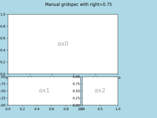
手動調整 GridSpec 配置#

當明確使用 GridSpec 時，您可以調整從 GridSpec 建立的子圖配置參數。請注意，此選項與受限配置或 Figure.tight_layout 不相容，這兩者都會忽略 left 和 right，並調整子圖大小以填滿圖形。通常，這種手動放置需要多次迭代才能使軸刻度標籤不與軸重疊。

這些間距參數也可以作為 gridspec_kw 引數傳遞給 subplots 和 subplot_mosaic。

fig = plt.figure(layout=None, facecolor='lightblue')
gs = fig.add_gridspec(nrows=3, ncols=3, left=0.05, right=0.75,
                      hspace=0.1, wspace=0.05)
ax0 = fig.add_subplot(gs[:-1, :])
annotate_axes(ax0, 'ax0')
ax1 = fig.add_subplot(gs[-1, :-1])
annotate_axes(ax1, 'ax1')
ax2 = fig.add_subplot(gs[-1, -1])
annotate_axes(ax2, 'ax2')
fig.suptitle('Manual gridspec with right=0.75')

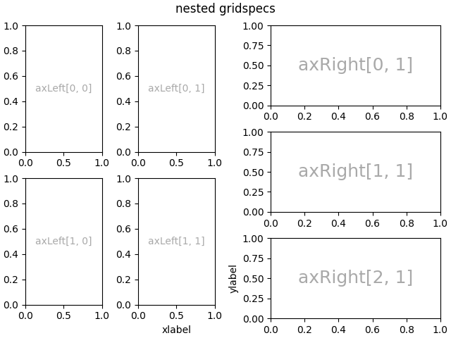
使用 SubplotSpec 的巢狀配置#

您可以使用 subgridspec 建立類似於 subfigures 的巢狀配置。此處的軸脊柱已對齊。

請注意，這也可從更詳細的 gridspec.GridSpecFromSubplotSpec 取得。

fig = plt.figure(layout="constrained")
gs0 = fig.add_gridspec(1, 2)

gs00 = gs0[0].subgridspec(2, 2)
gs01 = gs0[1].subgridspec(3, 1)

for a in range(2):
    for b in range(2):
        ax = fig.add_subplot(gs00[a, b])
        annotate_axes(ax, f'axLeft[{a}, {b}]', fontsize=10)
        if a == 1 and b == 1:
            ax.set_xlabel('xlabel')
for a in range(3):
    ax = fig.add_subplot(gs01[a])
    annotate_axes(ax, f'axRight[{a}, {b}]')
    if a == 2:
        ax.set_ylabel('ylabel')

fig.suptitle('nested gridspecs')

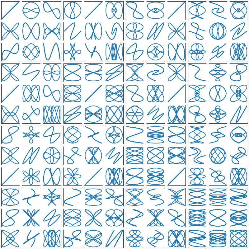
以下是一個更複雜的巢狀 GridSpec 範例：我們建立一個外部 4x4 格線，其中每個單元格都包含一個內部 3x3 軸格線。我們透過隱藏每個內部 3x3 格線中的適當脊柱來概述外部 4x4 格線。

def squiggle_xy(a, b, c, d, i=np.arange(0.0, 2*np.pi, 0.05)):
    return np.sin(i*a)*np.cos(i*b), np.sin(i*c)*np.cos(i*d)

fig = plt.figure(figsize=(8, 8), layout='constrained')
outer_grid = fig.add_gridspec(4, 4, wspace=0, hspace=0)

for a in range(4):
    for b in range(4):
        # gridspec inside gridspec
        inner_grid = outer_grid[a, b].subgridspec(3, 3, wspace=0, hspace=0)
        axs = inner_grid.subplots()  # Create all subplots for the inner grid.
        for (c, d), ax in np.ndenumerate(axs):
            ax.plot(*squiggle_xy(a + 1, b + 1, c + 1, d + 1))
            ax.set(xticks=[], yticks=[])

# show only the outside spines
for ax in fig.get_axes():
    ss = ax.get_subplotspec()
    ax.spines.top.set_visible(ss.is_first_row())
    ax.spines.bottom.set_visible(ss.is_last_row())
    ax.spines.left.set_visible(ss.is_first_col())
    ax.spines.right.set_visible(ss.is_last_col())

plt.show()