軸刻度

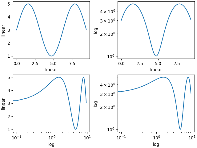
預設情況下，Matplotlib 使用線性刻度在軸上顯示資料。Matplotlib 也支援對數刻度，以及其他較不常見的刻度。通常，這可以直接使用 set_xscale 或 set_yscale 方法來完成。

import matplotlib.pyplot as plt
import numpy as np

import matplotlib.scale as mscale
from matplotlib.ticker import FixedLocator, NullFormatter

fig, axs = plt.subplot_mosaic([['linear', 'linear-log'],
                               ['log-linear', 'log-log']], layout='constrained')

x = np.arange(0, 3*np.pi, 0.1)
y = 2 * np.sin(x) + 3

ax = axs['linear']
ax.plot(x, y)
ax.set_xlabel('linear')
ax.set_ylabel('linear')

ax = axs['linear-log']
ax.plot(x, y)
ax.set_yscale('log')
ax.set_xlabel('linear')
ax.set_ylabel('log')

ax = axs['log-linear']
ax.plot(x, y)
ax.set_xscale('log')
ax.set_xlabel('log')
ax.set_ylabel('linear')

ax = axs['log-log']
ax.plot(x, y)
ax.set_xscale('log')
ax.set_yscale('log')
ax.set_xlabel('log')
ax.set_ylabel('log')

loglog 與 semilogx/y

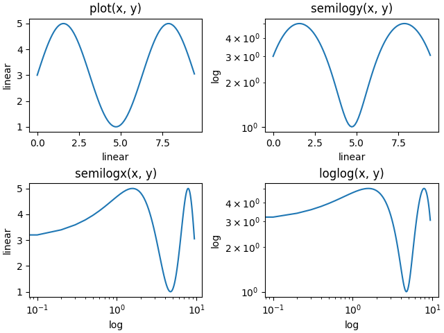
對數軸的使用非常頻繁，因此有一組輔助函數可以執行相同的操作：semilogy、semilogx 和 loglog。

fig, axs = plt.subplot_mosaic([['linear', 'linear-log'],
                               ['log-linear', 'log-log']], layout='constrained')

x = np.arange(0, 3*np.pi, 0.1)
y = 2 * np.sin(x) + 3

ax = axs['linear']
ax.plot(x, y)
ax.set_xlabel('linear')
ax.set_ylabel('linear')
ax.set_title('plot(x, y)')

ax = axs['linear-log']
ax.semilogy(x, y)
ax.set_xlabel('linear')
ax.set_ylabel('log')
ax.set_title('semilogy(x, y)')

ax = axs['log-linear']
ax.semilogx(x, y)
ax.set_xlabel('log')
ax.set_ylabel('linear')
ax.set_title('semilogx(x, y)')

ax = axs['log-log']
ax.loglog(x, y)
ax.set_xlabel('log')
ax.set_ylabel('log')
ax.set_title('loglog(x, y)')

其他內建刻度

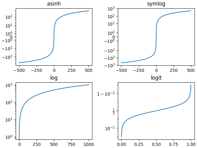
還有其他刻度可以使用。已註冊的刻度清單可以從 scale.get_scale_names 返回。

print(mscale.get_scale_names())

['asinh', 'function', 'functionlog', 'linear', 'log', 'logit', 'symlog']

fig, axs = plt.subplot_mosaic([['asinh', 'symlog'],
                               ['log', 'logit']], layout='constrained')

x = np.arange(0, 1000)

for name, ax in axs.items():
    if name in ['asinh', 'symlog']:
        yy = x - np.mean(x)
    elif name in ['logit']:
        yy = (x-np.min(x))
        yy = yy / np.max(np.abs(yy))
    else:
        yy = x

    ax.plot(yy, yy)
    ax.set_yscale(name)
    ax.set_title(name)

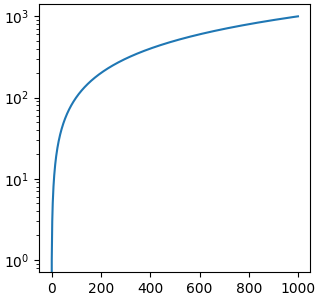
刻度的可選參數

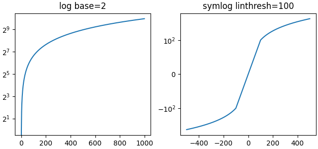
某些預設刻度具有可選參數。這些參數記錄在 scale 的各自刻度的 API 參考中。可以更改所繪製對數的基底（例如，以下為 2）或 'symlog' 的線性閾值範圍。

fig, axs = plt.subplot_mosaic([['log', 'symlog']], layout='constrained',
                              figsize=(6.4, 3))

for name, ax in axs.items():
    if name in ['log']:
        ax.plot(x, x)
        ax.set_yscale('log', base=2)
        ax.set_title('log base=2')
    else:
        ax.plot(x - np.mean(x), x - np.mean(x))
        ax.set_yscale('symlog', linthresh=100)
        ax.set_title('symlog linthresh=100')

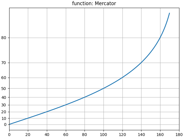
任意函數刻度

使用者可以定義完整的刻度類別，並將其傳遞給 set_xscale 和 set_yscale（請參閱 自訂刻度）。一個捷徑是使用 'function' 刻度，並傳遞 forward 和 inverse 函數作為額外參數。以下是對 y 軸執行 麥卡托投影。

# Function Mercator transform
def forward(a):
    a = np.deg2rad(a)
    return np.rad2deg(np.log(np.abs(np.tan(a) + 1.0 / np.cos(a))))


def inverse(a):
    a = np.deg2rad(a)
    return np.rad2deg(np.arctan(np.sinh(a)))


t = np.arange(0, 170.0, 0.1)
s = t / 2.

fig, ax = plt.subplots(layout='constrained')
ax.plot(t, s, '-', lw=2)

ax.set_yscale('function', functions=(forward, inverse))
ax.set_title('function: Mercator')
ax.grid(True)
ax.set_xlim([0, 180])
ax.yaxis.set_minor_formatter(NullFormatter())
ax.yaxis.set_major_locator(FixedLocator(np.arange(0, 90, 10)))

什麼是「刻度」？

刻度是一個附加到軸的物件。類別文件位於 scale。set_xscale 和 set_yscale 在各自的軸物件上設定刻度。您可以使用 get_scale 確定軸上的刻度

fig, ax = plt.subplots(layout='constrained',
                              figsize=(3.2, 3))
ax.semilogy(x, x)

print(ax.xaxis.get_scale())
print(ax.yaxis.get_scale())

linear
log

設定刻度會執行三件事。首先，它會在軸上定義一個轉換，該轉換會在資料值和沿軸的位置之間進行對應。此轉換可以透過 get_transform 存取

print(ax.yaxis.get_transform())

LogTransform(base=10, nonpositive='clip')

軸上的轉換是一個相對底層的概念，但它是 set_scale 所扮演的重要角色之一。

設定刻度也會為刻度設定預設的刻度定位器 (ticker) 和刻度格式器。具有 'log' 刻度的軸具有 LogLocator，用於選擇十進位間隔的刻度，以及 LogFormatter，用於在十進位數上使用科學記號。

print('X axis')
print(ax.xaxis.get_major_locator())
print(ax.xaxis.get_major_formatter())

print('Y axis')
print(ax.yaxis.get_major_locator())
print(ax.yaxis.get_major_formatter())

X axis
<matplotlib.ticker.AutoLocator object at 0x7e4c95c76270>
<matplotlib.ticker.ScalarFormatter object at 0x7e4c95c74f20>
Y axis
<matplotlib.ticker.LogLocator object at 0x7e4c938944d0>
<matplotlib.ticker.LogFormatterSciNotation object at 0x7e4c95b84200>