Matplotlib 3.6.0 的新功能 (2022 年 9 月 15 日)#
如需上次修訂以來所有問題和提取請求的清單,請參閱3.10.0 (2024 年 12 月 13 日) 的 GitHub 統計數據。
圖表和軸的建立/管理#
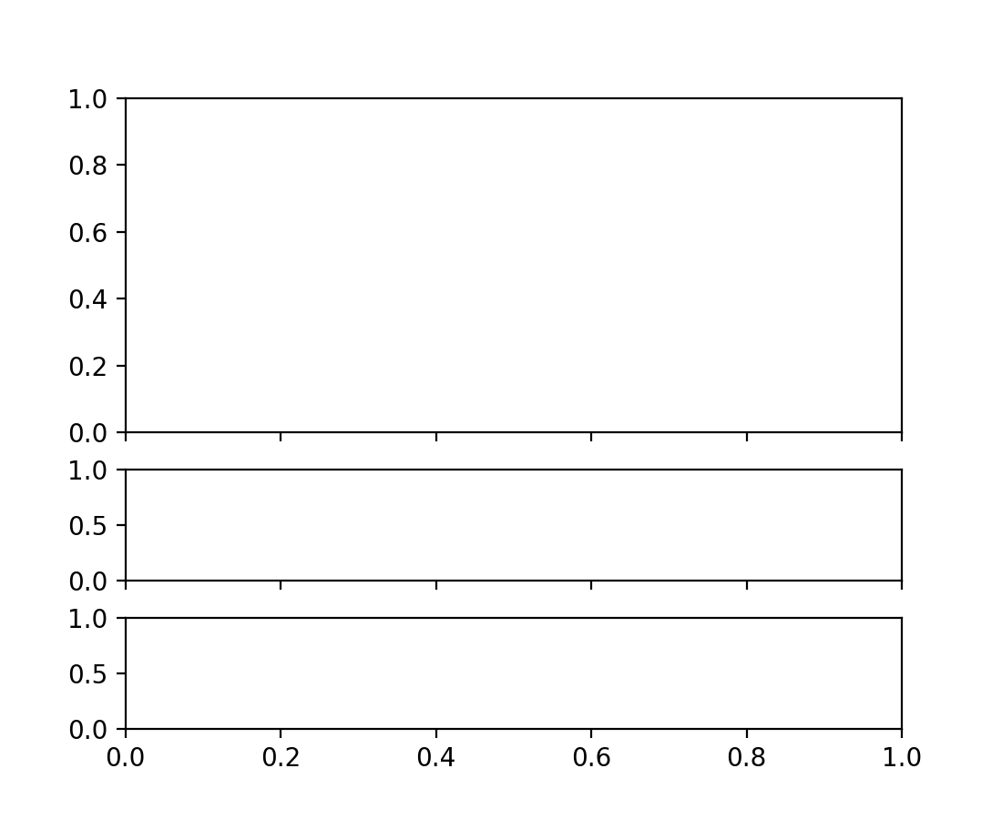
subplots, subplot_mosaic 接受 height_ratios 和 width_ratios 引數#
在 subplots 和 subplot_mosaic 中,欄和列的相對寬度和高度可以透過將 height_ratios 和 width_ratios 關鍵字引數傳遞給這些方法來控制。
fig = plt.figure()
axs = fig.subplots(3, 1, sharex=True, height_ratios=[3, 1, 1])
先前,這需要將比例傳遞到 gridspec_kw 引數中
fig = plt.figure()
axs = fig.subplots(3, 1, sharex=True,
                   gridspec_kw=dict(height_ratios=[3, 1, 1]))
約束式佈局不再被視為實驗性功能#
約束式佈局引擎和 API 不再被視為實驗性。在沒有棄用期的情況下,不再允許任意變更行為和 API。
新的 layout_engine 模組#
Matplotlib 附帶 tight_layout 和 constrained_layout 佈局引擎。提供了一個新的 layout_engine 模組,允許下游函式庫編寫自己的佈局引擎,並且 Figure 物件現在可以接受 LayoutEngine 子類別作為 layout 參數的引數。
用於固定縱橫比軸的壓縮佈局#
現在可以使用 fig, axs = plt.subplots(2, 3, layout='compressed') 將具有固定縱橫比的軸的簡單排列組裝在一起。
使用 layout='tight' 或 'constrained',具有固定縱橫比的軸之間可能會留下很大的間隙
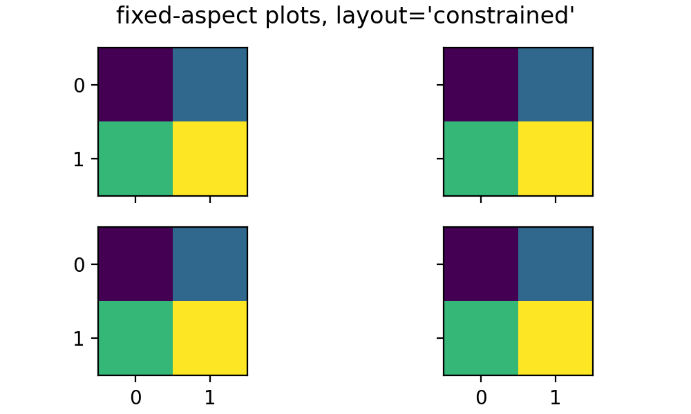
使用 layout='compressed' 佈局會減少軸之間的空間,並將額外的空間添加到外部邊距
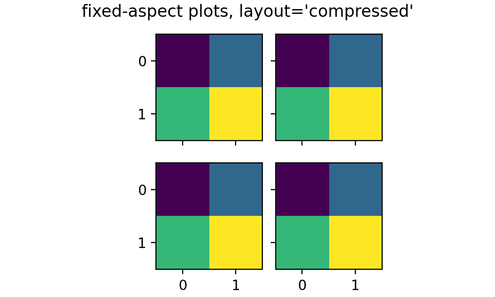
有關詳細資訊,請參閱固定縱橫比軸的網格: "壓縮" 佈局。
現在可以移除佈局引擎#
現在可以透過使用 'none' 呼叫 Figure.set_layout_engine 來移除圖表上的佈局引擎。這在計算佈局後可能很有用,以減少計算量,例如,用於後續的動畫迴圈。
之後可以設定不同的佈局引擎,只要它與先前的佈局引擎相容即可。
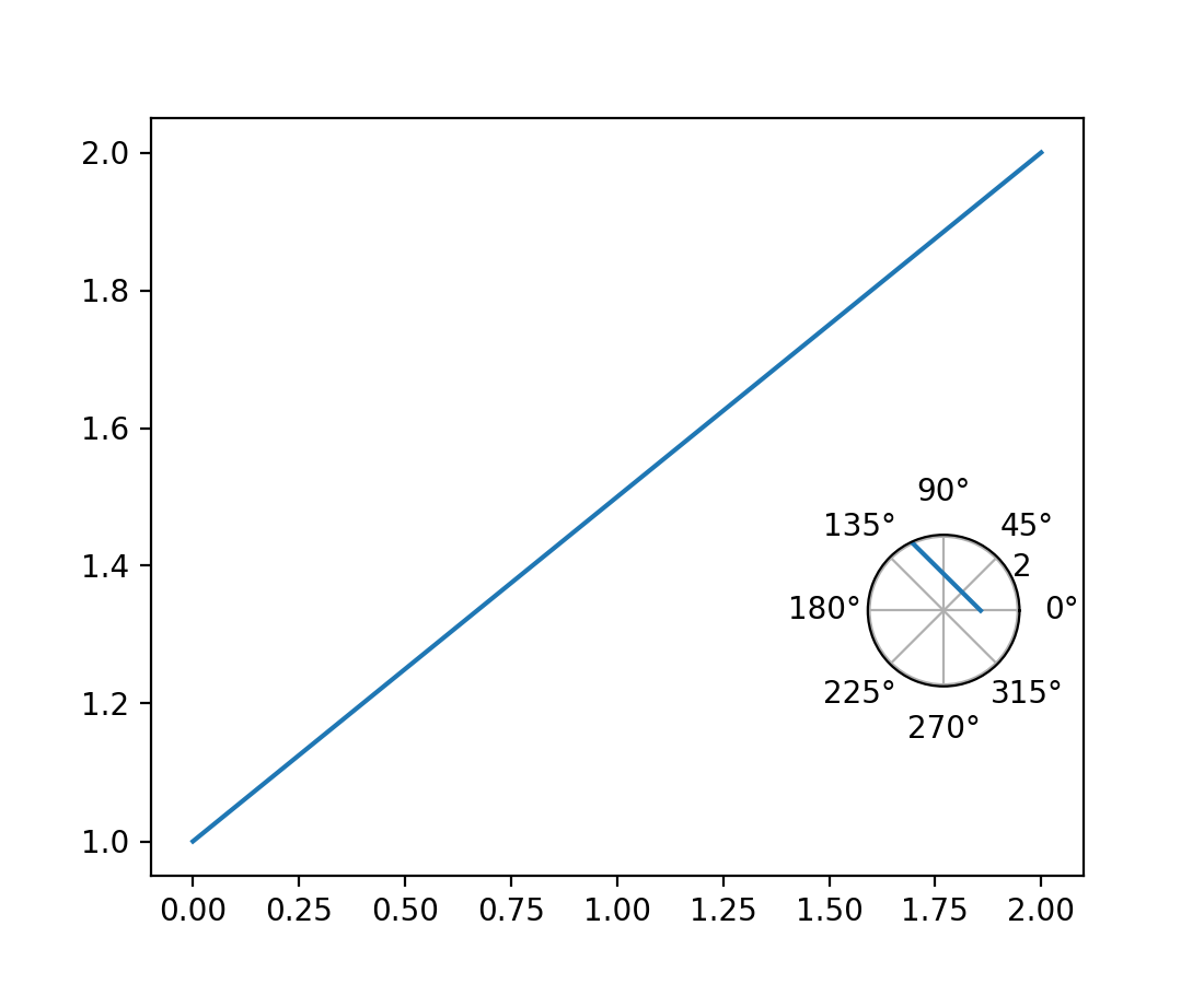
Axes.inset_axes 的彈性#
matplotlib.axes.Axes.inset_axes 現在接受 projection、polar 和 axes_class 關鍵字引數,以便可以傳回 matplotlib.axes.Axes 的子類別。
fig, ax = plt.subplots()

ax.plot([0, 2], [1, 2])

polar_ax = ax.inset_axes([0.75, 0.25, 0.2, 0.2], projection='polar')
polar_ax.plot([0, 2], [1, 2])
WebP 現在是一種支援的輸出格式#
現在可以使用 .webp 副檔名,或將 format='webp' 傳遞給 savefig,以 WebP 格式儲存圖表。這依賴於 Pillow 對 WebP 的支援。
圖表關閉時不再執行垃圾收集#
Matplotlib 有大量的循環引用(在圖表和管理員之間、在軸和圖表之間、軸和藝術家之間、圖表和畫布之間等),因此當使用者刪除他們對圖表的最後一個引用(並從 pyplot 的狀態中清除它)時,物件不會立即被刪除。
為了解決這個問題,我們長期以來(自 2004 年之前)在關閉程式碼中使用了 gc.collect(僅限最低的兩個世代),以便及時清理自身。然而,這既沒有達到我們想要的效果(因為我們的大多數物件實際上會保留下來),而且由於清除了第一代,我們也打開了無限制記憶體使用的可能性。
在建立圖表和銷毀圖表之間有非常緊密的迴圈的情況下(例如 plt.figure(); plt.close()),第一代永遠不會變得足夠大,讓 Python 考慮在較高的世代上執行收集。這將導致無限制的記憶體使用,因為長壽命的物件永遠不會被重新考慮以尋找引用循環,因此永遠不會被刪除。
我們現在在關閉圖表時不再執行任何垃圾收集,而是依賴 Python 自動決定定期執行垃圾收集。如果您有嚴格的記憶體需求,您可以自己呼叫 gc.collect,但這可能會在緊密的計算迴圈中產生效能影響。
繪圖方法#
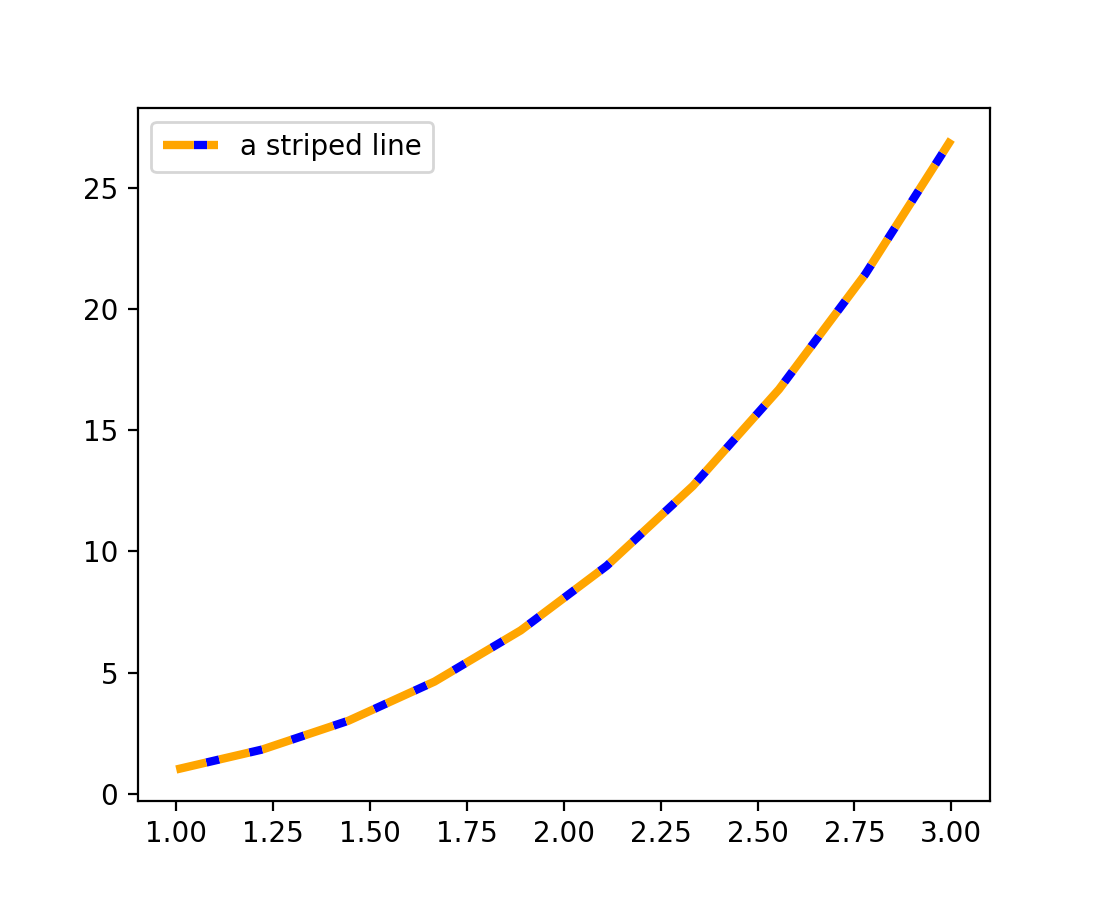
條紋線 (實驗性)#
plot 的新 gapcolor 參數可以建立條紋線。
x = np.linspace(1., 3., 10)
y = x**3

fig, ax = plt.subplots()
ax.plot(x, y, linestyle='--', color='orange', gapcolor='blue',
        linewidth=3, label='a striped line')
ax.legend()
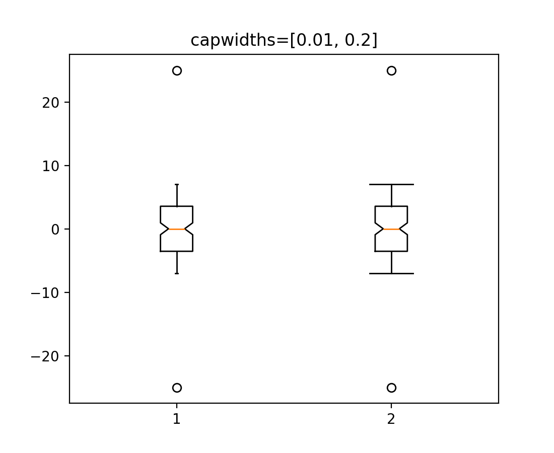
在 bxp 和 boxplot 中,箱形圖和鬚狀圖的自訂帽寬#
新的 capwidths 參數加入到 bxp 和 boxplot 中,可以控制箱形圖和鬚狀圖中帽子的寬度。
x = np.linspace(-7, 7, 140)
x = np.hstack([-25, x, 25])
capwidths = [0.01, 0.2]

fig, ax = plt.subplots()
ax.boxplot([x, x], notch=True, capwidths=capwidths)
ax.set_title(f'{capwidths=}')
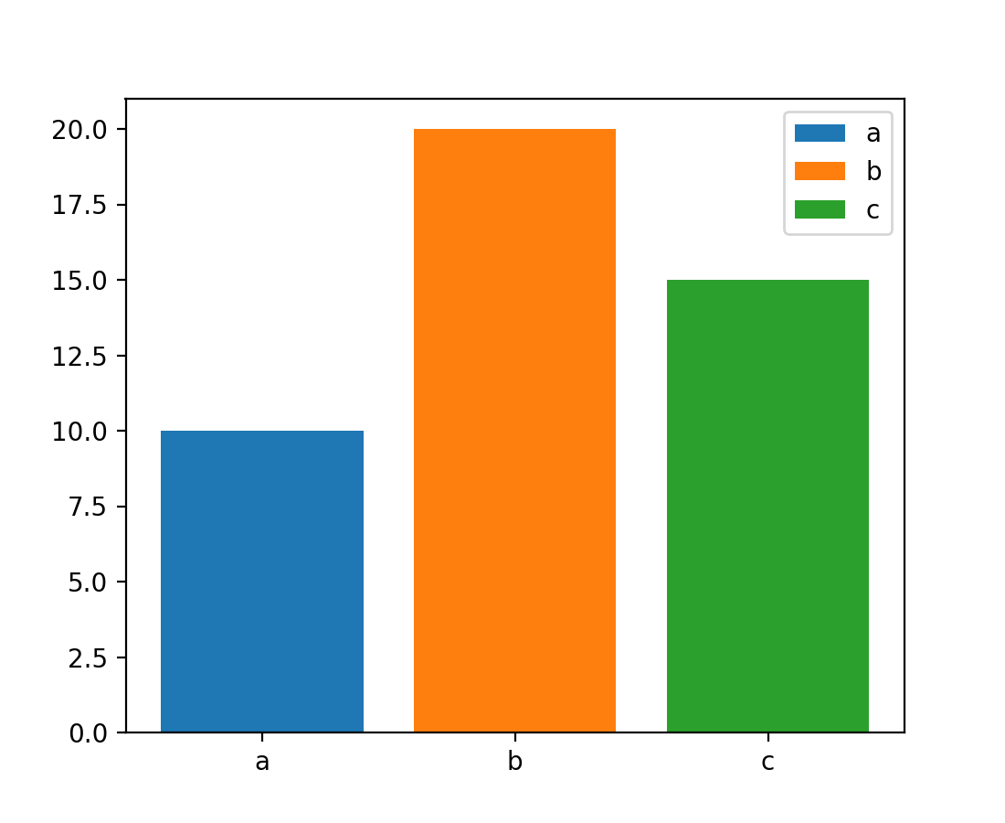
長條圖中更簡易的標籤設定#
bar 和 barh 的 label 參數現在可以傳入長條標籤的列表。該列表的長度必須與 x 相同,並為各個長條加上標籤。重複的標籤不會被去重,並將導致重複的標籤項目,因此最好在長條的樣式也不同時使用(例如,將列表傳遞給 color,如下所示。)
x = ["a", "b", "c"]
y = [10, 20, 15]
color = ['C0', 'C1', 'C2']

fig, ax = plt.subplots()
ax.bar(x, y, color=color, label=x)
ax.legend()
顏色條刻度的新樣式格式字串#
colorbar (和其他顏色條方法) 的 format 參數現在接受 {} 樣式的格式字串。
fig, ax = plt.subplots()
im = ax.imshow(z)
fig.colorbar(im, format='{x:.2e}')  # Instead of '%.2e'
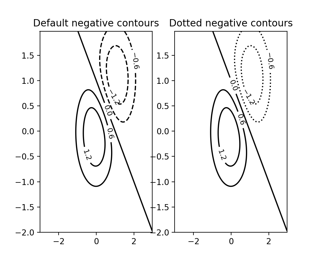
負等高線的線條樣式可以單獨設定#
負等高線的線條樣式可以通過將 negative_linestyles 參數傳遞給 Axes.contour 來設定。之前,此樣式只能通過 rcParams["contour.negative_linestyle"] (預設值:'dashed') 全域設定。
delta = 0.025
x = np.arange(-3.0, 3.0, delta)
y = np.arange(-2.0, 2.0, delta)
X, Y = np.meshgrid(x, y)
Z1 = np.exp(-X**2 - Y**2)
Z2 = np.exp(-(X - 1)**2 - (Y - 1)**2)
Z = (Z1 - Z2) * 2

fig, axs = plt.subplots(1, 2)

CS = axs[0].contour(X, Y, Z, 6, colors='k')
axs[0].clabel(CS, fontsize=9, inline=True)
axs[0].set_title('Default negative contours')

CS = axs[1].contour(X, Y, Z, 6, colors='k', negative_linestyles='dotted')
axs[1].clabel(CS, fontsize=9, inline=True)
axs[1].set_title('Dotted negative contours')
通過 ContourPy 改善四邊形等高線計算#
等高線函數 contour 和 contourf 有一個新的關鍵字參數 algorithm,用於控制計算等高線所使用的演算法。有四種演算法可供選擇,預設是使用 algorithm='mpl2014',這是 Matplotlib 自 2014 年以來一直在使用的相同演算法。
先前,Matplotlib 使用自己的 C++ 程式碼來計算四邊形網格的等高線。現在改為使用外部函式庫 ContourPy。
目前 algorithm 關鍵字參數的其他可能值為 'mpl2005'、'serial' 和 'threaded';有關詳細資訊,請參閱 ContourPy 文件。
注意
由 algorithm='mpl2014' 產生的等高線和多邊形將與此變更之前產生的等高線和多邊形相同,僅在浮點數精確度的容差範圍內有差異。唯一的例外是重複點,即包含相鄰的相同 (x, y) 點的等高線;之前,重複的點被移除,現在則保留。受此影響的等高線將產生相同的視覺輸出,但等高線中的點數會更多。
使用 clabel 取得的等高線標籤位置也可能不同。
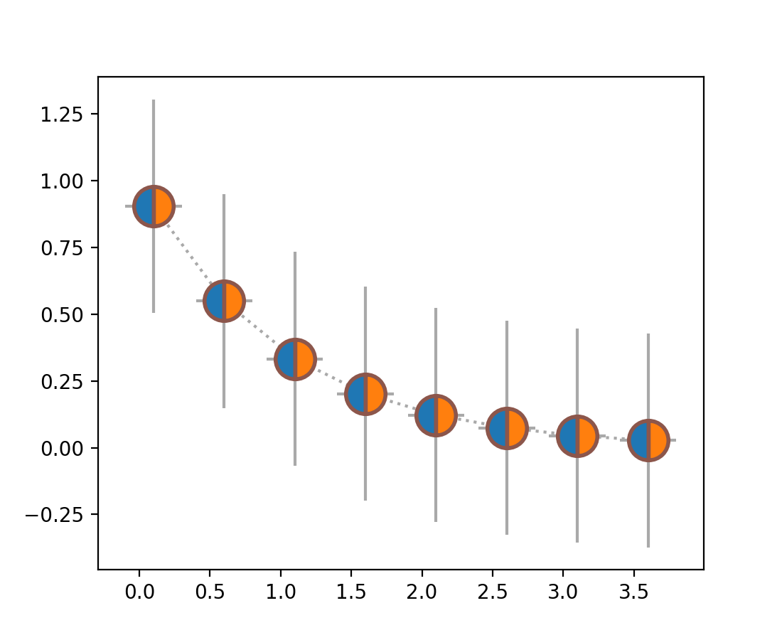
errorbar 支援 markerfacecoloralt#
markerfacecoloralt 參數現在會從 Axes.errorbar 傳遞給線條繪圖器。文件現在正確列出哪些屬性被傳遞到 Line2D,而不是聲稱所有關鍵字參數都會被傳遞。
x = np.arange(0.1, 4, 0.5)
y = np.exp(-x)

fig, ax = plt.subplots()
ax.errorbar(x, y, xerr=0.2, yerr=0.4,
            linestyle=':', color='darkgrey',
            marker='o', markersize=20, fillstyle='left',
            markerfacecolor='tab:blue', markerfacecoloralt='tab:orange',
            markeredgecolor='tab:brown', markeredgewidth=2)
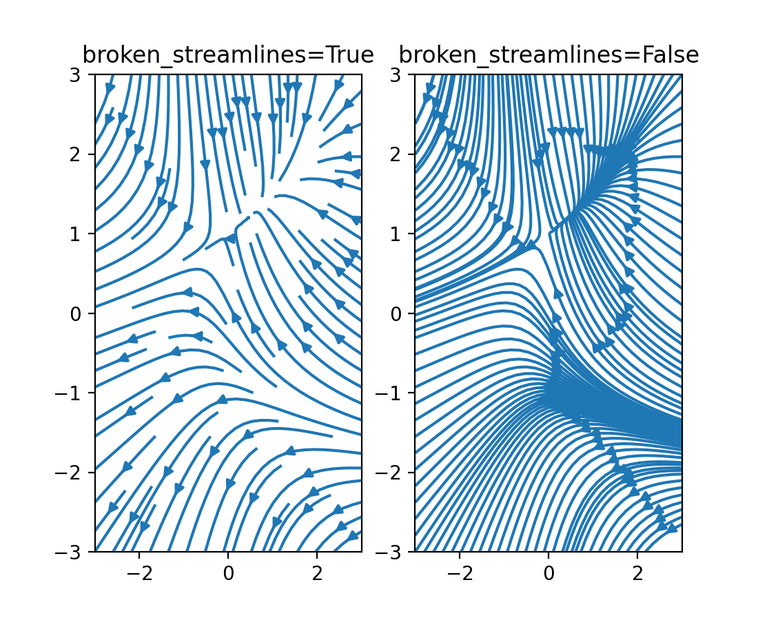
streamplot 可以停用流線中斷#
現在可以指定流線圖具有連續且不斷裂的流線。先前,流線會結束以限制單個網格單元中的線條數量。請參閱以下圖表之間的差異
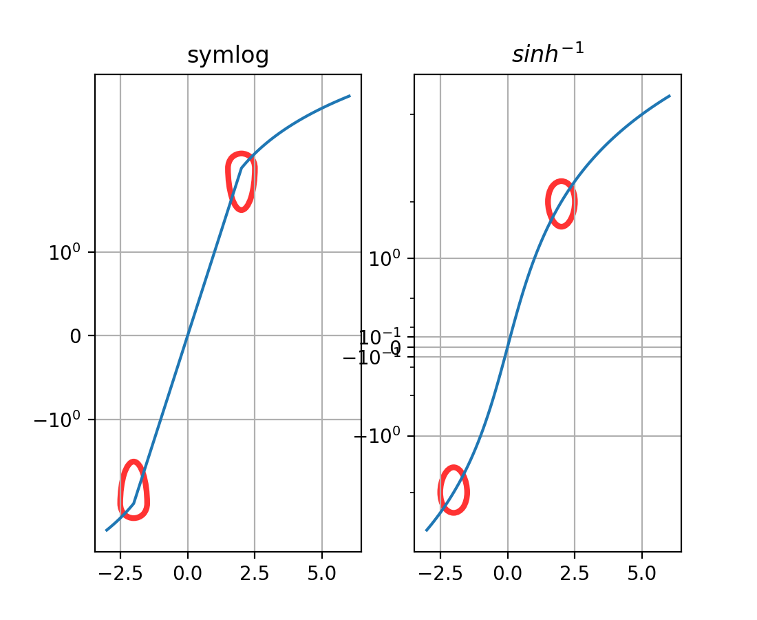
新的軸刻度 asinh (實驗性)#
新的 asinh 軸刻度提供 symlog 的替代方案,可以在刻度的準線性區域和漸近對數區域之間平滑過渡。這是基於 arcsinh 轉換,允許繪製跨越多個數量級的正值和負值。
stairs(..., fill=True) 通過設定線寬來隱藏邊緣#
stairs(..., fill=True) 之前會透過設定 edgecolor="none" 來隱藏 Patch 邊緣。因此,稍後在 Patch 上調用 set_color() 會使 Patch 顯得更大。
現在,透過使用 linewidth=0,可以防止這種明顯的尺寸變化。同樣地,呼叫 stairs(..., fill=True, linewidth=3) 的行為將更加透明。
修正 Patch 類的虛線偏移#
先前,在使用虛線元組設定 Patch 物件上的線條樣式時,會忽略偏移。現在,偏移會如預期地應用於 Patch,並且可以像使用 Line2D 物件一樣使用。
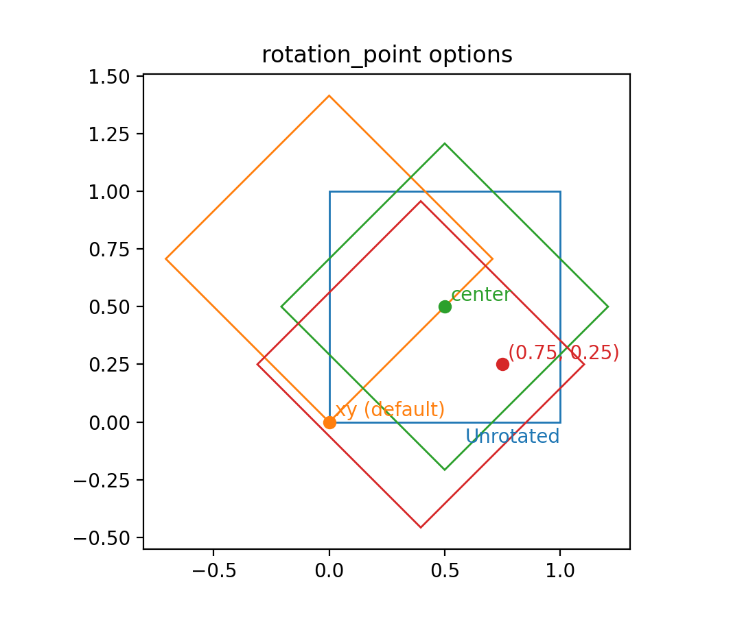
矩形 Patch 旋轉點#
現在可以使用 rotation_point 參數將 Rectangle 的旋轉點設定為 'xy'、'center' 或包含兩個數字的元組。
顏色和色彩對應#
顏色序列註冊表#
顏色序列註冊表,ColorSequenceRegistry,包含 Matplotlib 已知名稱的顏色序列(即簡單的列表)。通常不會直接使用此註冊表,而是透過 matplotlib.color_sequences 的通用實例來使用。
用於建立不同大小查找表的 Colormap 方法#
新的方法 Colormap.resampled 會建立一個新的 Colormap 實例,其具有指定的查找表大小。這是透過 get_cmap 操作查找表大小的替代方案。
使用
get_cmap(name).resampled(N)
取代
get_cmap(name, lut=N)
使用字串設定 Norms#
現在可以使用對應比例的字串名稱來設定 Norms(例如在圖像上),例如 imshow(array, norm="log")。請注意,在這種情況下,也可以傳遞 *vmin* 和 *vmax*,因為在底層會建立一個新的 Norm 實例。
標題、刻度和標籤#
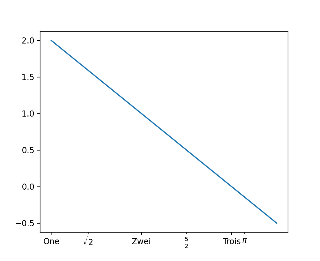
plt.xticks 和 plt.yticks 支援 minor 關鍵字參數#
現在可以透過設定 minor=True,使用 pyplot.xticks 和 pyplot.yticks 來設定或取得次要刻度。
plt.figure()
plt.plot([1, 2, 3, 3.5], [2, 1, 0, -0.5])
plt.xticks([1, 2, 3], ["One", "Zwei", "Trois"])
plt.xticks([np.sqrt(2), 2.5, np.pi],
           [r"$\sqrt{2}$", r"$\frac{5}{2}$", r"$\pi$"], minor=True)
圖例#
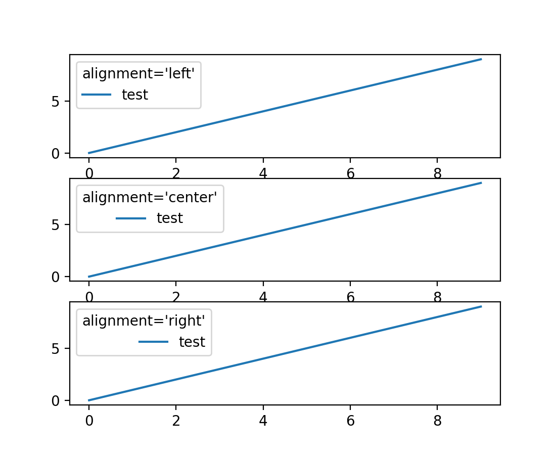
圖例可以控制標題和圖柄的對齊方式#
Legend 現在支援透過關鍵字參數 *alignment* 來控制標題和圖柄的對齊方式。您也可以使用 Legend.set_alignment 來控制現有圖例的對齊方式。
fig, axs = plt.subplots(3, 1)
for i, alignment in enumerate(['left', 'center', 'right']):
    axs[i].plot(range(10), label='test')
    axs[i].legend(title=f'{alignment=}', alignment=alignment)
legend 的 ncol 關鍵字參數已重新命名為 ncols#
用於控制列數的 legend 的 ncol 關鍵字參數已重新命名為 ncols,以與 subplots 和 GridSpec 的 ncols 和 nrows 關鍵字保持一致。為了向後相容,仍然支援 ncol,但不建議使用。
標記#
marker 現在可以設定為字串 "none"#
字串 "none" 表示*無標記*,與其他支援小寫版本的 API 一致。建議使用 "none" 而不是 "None",以避免與 None 物件混淆。
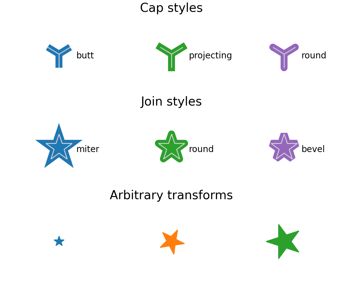
自訂 MarkerStyle 連接和端點樣式#
新的 MarkerStyle 參數允許控制連接樣式和端點樣式,並讓使用者提供要套用至標記的轉換(例如旋轉)。
from matplotlib.markers import CapStyle, JoinStyle, MarkerStyle
from matplotlib.transforms import Affine2D

fig, axs = plt.subplots(3, 1, layout='constrained')
for ax in axs:
    ax.axis('off')
    ax.set_xlim(-0.5, 2.5)

axs[0].set_title('Cap styles', fontsize=14)
for col, cap in enumerate(CapStyle):
    axs[0].plot(col, 0, markersize=32, markeredgewidth=8,
                marker=MarkerStyle('1', capstyle=cap))
    # Show the marker edge for comparison with the cap.
    axs[0].plot(col, 0, markersize=32, markeredgewidth=1,
                markerfacecolor='none', markeredgecolor='lightgrey',
                marker=MarkerStyle('1'))
    axs[0].annotate(cap.name, (col, 0),
                    xytext=(20, -5), textcoords='offset points')

axs[1].set_title('Join styles', fontsize=14)
for col, join in enumerate(JoinStyle):
    axs[1].plot(col, 0, markersize=32, markeredgewidth=8,
                marker=MarkerStyle('*', joinstyle=join))
    # Show the marker edge for comparison with the join.
    axs[1].plot(col, 0, markersize=32, markeredgewidth=1,
                markerfacecolor='none', markeredgecolor='lightgrey',
                marker=MarkerStyle('*'))
    axs[1].annotate(join.name, (col, 0),
                    xytext=(20, -5), textcoords='offset points')

axs[2].set_title('Arbitrary transforms', fontsize=14)
for col, (size, rot) in enumerate(zip([2, 5, 7], [0, 45, 90])):
    t = Affine2D().rotate_deg(rot).scale(size)
    axs[2].plot(col, 0, marker=MarkerStyle('*', transform=t))
字體和文字#
字體回退#
現在可以指定字體系列的列表,Matplotlib 會按順序嘗試它們以找到所需的字形。
plt.rcParams["font.size"] = 20
fig = plt.figure(figsize=(4.75, 1.85))

text = "There are 几个汉字 in between!"
fig.text(0.05, 0.65, text, family=["Noto Sans CJK JP", "Noto Sans TC"])
fig.text(0.05, 0.45, text, family=["DejaVu Sans", "Noto Sans CJK JP", "Noto Sans TC"])
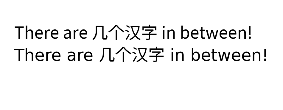
示範混合英文和中文文字與字體回退。
這目前適用於 Agg(和所有 GUI 嵌入)、svg、pdf、ps 和內嵌後端。
可用的字體名稱列表#
現在可以輕鬆存取可用字體的列表。若要取得 Matplotlib 中可用字體名稱的列表,請使用
from matplotlib import font_manager
font_manager.get_font_names()
math_to_image 現在具有 color 關鍵字參數#
為了輕鬆支援依賴 Matplotlib 的 MathText 渲染來產生方程式圖像的外部程式庫,math_to_image 中新增了 color 關鍵字參數。
from matplotlib import mathtext
mathtext.math_to_image('$x^2$', 'filename.png', color='Maroon')
活動 URL 區域會隨著連結文字旋轉#
當圖形中的連結文字旋轉時,活動 URL 區域現在會包含旋轉的連結區域。先前,活動區域保持在原始的、未旋轉的位置。
rcParams 改進#
允許全域設定圖形標籤的大小和粗細,並與標題分開#
對於圖形標籤,Figure.supxlabel 和 Figure.supylabel,可以使用 rcParams["figure.labelsize"](預設值:'large')和 rcParams["figure.labelweight"](預設值:'normal')來設定其大小和粗細,使其與圖形標題分開。
# Original (previously combined with below) rcParams:
plt.rcParams['figure.titlesize'] = 64
plt.rcParams['figure.titleweight'] = 'bold'

# New rcParams:
plt.rcParams['figure.labelsize'] = 32
plt.rcParams['figure.labelweight'] = 'bold'

fig, axs = plt.subplots(2, 2, layout='constrained')
for ax in axs.flat:
    ax.set(xlabel='xlabel', ylabel='ylabel')

fig.suptitle('suptitle')
fig.supxlabel('supxlabel')
fig.supylabel('supylabel')
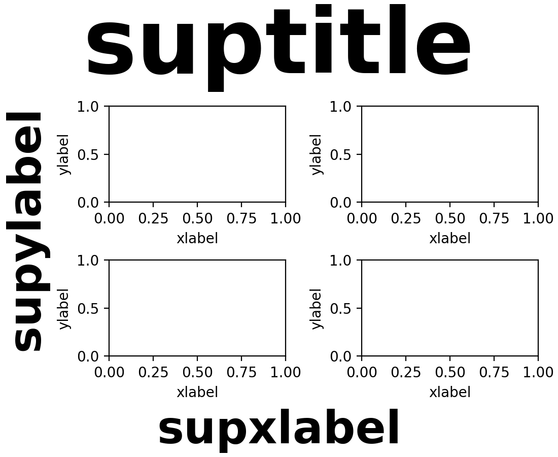
請注意,如果您已變更 rcParams["figure.titlesize"] (預設值:'large') 或 rcParams["figure.titleweight"] (預設值:'normal'),您現在也必須變更新引入的參數,才能獲得與過去行為一致的結果。
Mathtext 剖析可以全域停用#
可以使用 rcParams["text.parse_math"] (預設值:True) 設定來停用所有 Text 物件中的 mathtext 剖析 (最明顯的是來自 Axes.text 方法)。
matplotlibrc 中的雙引號字串#
您現在可以在字串周圍使用雙引號。這允許在字串中使用 '#' 字元。在沒有引號的情況下,'#' 會被解釋為註解的開始。特別是,您現在可以定義十六進位顏色:
grid.color: "#b0b0b0"
3D 軸線的改進#
主要平面視角的標準化視圖#
當在主要視圖平面 (即垂直於 XY、XZ 或 YZ 平面) 中檢視 3D 繪圖時,軸線將會顯示在標準位置。有關 3D 視圖的詳細資訊,請參閱 mplot3d 視角 和 主要 3D 視圖平面。
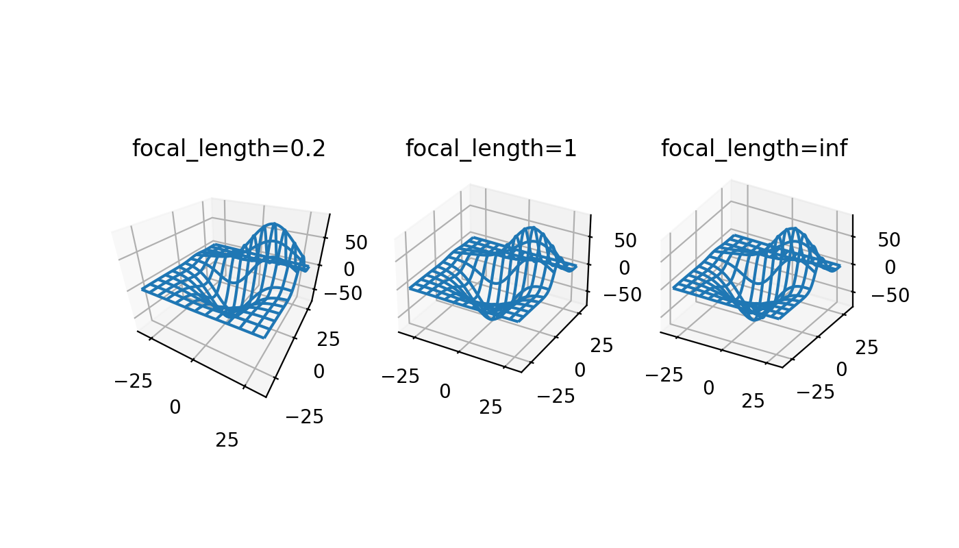
3D 相機的自訂焦距#
現在可以透過指定虛擬相機的焦距,使 3D 軸線更好地模擬真實世界的相機。預設焦距 1 對應於 90° 的視場 (FOV),並且與現有的 3D 繪圖向後相容。介於 1 和無限大之間的增加焦距會「展平」影像,而介於 1 和 0 之間的減少焦距則會誇大透視效果,並使影像具有更明顯的深度。
焦距可以透過以下方程式從所需的 FOV 計算得出:

from mpl_toolkits.mplot3d import axes3d

X, Y, Z = axes3d.get_test_data(0.05)

fig, axs = plt.subplots(1, 3, figsize=(7, 4),
                        subplot_kw={'projection': '3d'})

for ax, focal_length in zip(axs, [0.2, 1, np.inf]):
    ax.plot_wireframe(X, Y, Z, rstride=10, cstride=10)
    ax.set_proj_type('persp', focal_length=focal_length)
    ax.set_title(f"{focal_length=}")
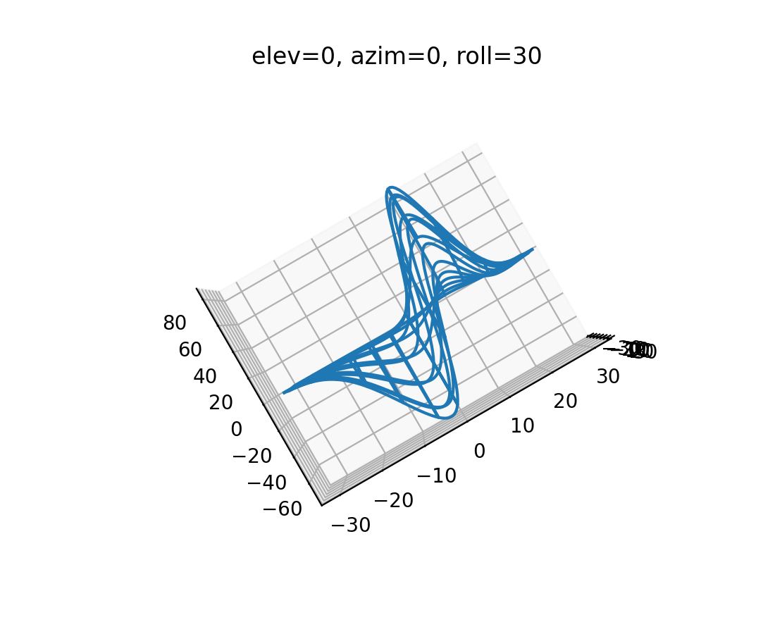
3D 繪圖新增了第三個「滾動」視角#
現在可以透過新增第三個滾動角度從任何方向檢視 3D 繪圖,該角度會繞著檢視軸旋轉繪圖。使用滑鼠的互動式旋轉仍然僅控制仰角和方位角,這表示此功能與以程式設計方式建立更複雜的相機角度的使用者相關。預設滾動角度 0 與現有的 3D 繪圖向後相容。
from mpl_toolkits.mplot3d import axes3d

X, Y, Z = axes3d.get_test_data(0.05)

fig, ax = plt.subplots(subplot_kw={'projection': '3d'})

ax.plot_wireframe(X, Y, Z, rstride=10, cstride=10)
ax.view_init(elev=0, azim=0, roll=30)
ax.set_title('elev=0, azim=0, roll=30')
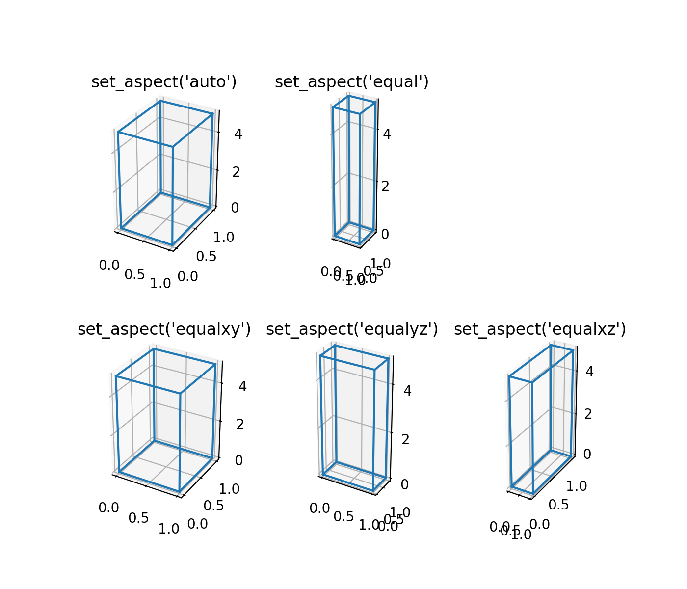
3D 繪圖的等比例#
使用者可以將 3D 繪圖的 X、Y、Z 軸的比例設定為「相等」、「equalxy」、「equalxz」或「equalyz」,而不是預設的「自動」。
from itertools import combinations, product

aspects = [
    ['auto', 'equal', '.'],
    ['equalxy', 'equalyz', 'equalxz'],
]
fig, axs = plt.subplot_mosaic(aspects, figsize=(7, 6),
                              subplot_kw={'projection': '3d'})

# Draw rectangular cuboid with side lengths [1, 1, 5]
r = [0, 1]
scale = np.array([1, 1, 5])
pts = combinations(np.array(list(product(r, r, r))), 2)
for start, end in pts:
    if np.sum(np.abs(start - end)) == r[1] - r[0]:
        for ax in axs.values():
            ax.plot3D(*zip(start*scale, end*scale), color='C0')

# Set the aspect ratios
for aspect, ax in axs.items():
    ax.set_box_aspect((3, 4, 5))
    ax.set_aspect(aspect)
    ax.set_title(f'set_aspect({aspect!r})')
互動式工具的改進#
旋轉、比例校正和新增/移除狀態#
現在可以在 -45° 和 45° 之間互動式旋轉 RectangleSelector 和 EllipseSelector。範圍限制目前由實作決定。可以透過按下 r 鍵 (「r」是預設對應於 state_modifier_keys 中的「旋轉」的按鍵) 或呼叫 selector.add_state('rotate') 來啟用或停用旋轉。
現在在使用「正方形」狀態時,可以將軸線的比例納入考量。這可以透過在初始化選取器時指定 use_data_coordinates='True' 來啟用。
除了使用 state_modifier_keys 中定義的修飾鍵互動式變更選取器狀態之外,現在也可以使用 add_state 和 remove_state 方法以程式設計方式變更選取器狀態。
from matplotlib.widgets import RectangleSelector

values = np.arange(0, 100)

fig = plt.figure()
ax = fig.add_subplot()
ax.plot(values, values)

selector = RectangleSelector(ax, print, interactive=True,
                             drag_from_anywhere=True,
                             use_data_coordinates=True)
selector.add_state('rotate')  # alternatively press 'r' key
# rotate the selector interactively

selector.remove_state('rotate')  # alternatively press 'r' key

selector.add_state('square')
MultiCursor 現在支援跨多個圖形的軸線分割#
先前,MultiCursor 僅在所有目標軸線都屬於同一個圖形時才有效。
由於這項變更,MultiCursor 建構函式的第一個引數已變成未使用 (先前它是所有軸線的聯合畫布,但畫布現在直接從軸線清單中推斷)。
PolygonSelector 邊界框#
PolygonSelector 現在有一個 draw_bounding_box 引數,當設定為 True 時,會在多邊形完成後在其周圍繪製一個邊界框。可以調整邊界框的大小和移動它,以便輕鬆調整多邊形的點的大小。
設定 PolygonSelector 頂點#
現在可以使用 PolygonSelector.verts 屬性以程式設計方式設定 PolygonSelector 的頂點。以這種方式設定頂點會重設選取器,並使用提供的頂點建立新的完整選取器。
SpanSelector 小工具現在可以快取至指定的值#
現在可以將 SpanSelector 小工具快取至 snap_values 引數指定的值。
更多工具列圖示針對深色主題進行樣式設定#
在 macOS 和 Tk 後端上,使用深色主題時,工具列圖示現在會反轉。
平台特定變更#
Wx 後端使用標準工具列#
工具列設定在 Wx 視窗上作為標準工具列,而不是自訂的大小調整器。
macosx 後端的改進#
修飾鍵的處理更加一致#
macosx 後端現在以與其他後端更一致的方式處理修飾鍵。如需更多資訊,請參閱 事件連線 中的表格。
savefig.directory rcParam 支援#
macosx 後端現在會遵守 rcParams["savefig.directory"] (預設值:'~') 設定。如果設定為非空字串,則儲存對話方塊會預設為此目錄,並保留後續儲存目錄的變更。
figure.raise_window rcParam 支援#
macosx 後端現在會遵守 rcParams["figure.raise_window"] (預設值:True) 設定。如果設定為 False,圖形視窗在更新時不會被帶到最上層。
全螢幕切換支援#
如同其他後端所支援的,macosx 後端現在也支援切換全螢幕檢視。預設情況下,可以按下 f 鍵來切換此檢視。
改進的動畫和位元區塊傳輸支援#
macosx 後端已進行改進,以修復位元區塊傳輸、包含新繪圖器的動畫影格,並減少不必要的繪圖呼叫。
macOS 應用程式圖示已套用至 Qt 後端#
當在 macOS 上使用基於 Qt 的後端時,應用程式圖示現在會被設定,如同在其他後端/平台上所做的一樣。
新的最低 macOS 版本#
macosx 後端現在需要 macOS >= 10.12。
Windows on ARM 支援#
已新增針對 arm64 目標的 Windows 的初步支援。此支援需要 FreeType 2.11 或更高版本。
目前尚無可用的二進位 wheel 檔,但可以從原始碼建置。